
Introduction to storage performance analysis with PCP
This article is an introduction and tutorial on basic storage performance analysis tasks using Performance Co-Pilot (PCP).
INTRODUCTION
Performance Co-Pilot is a system level performance monitoring and management suite, particularly suited for use in enterprise environments. PCP has shipped and been fully supported by Red Hat since RHEL 6.6 and in many other distributions (e.g. Fedora since F15, Debian, Ubuntu, etc.). It's a stable, actively maintained and developed open source project, with a supportive community, see the PCP Home Page and the project page on GITHUB and the git repo.

- Metrics coverage - PCP captures just about everything exported by the Linux /proc and /sys pseudo filesystems, including per-process data. PCP is easily extensible and has 96 plugins available (at last count), e.g. Linux platform, Oracle, mmv (for Java/JVM), libvirt, container support and many many others, with new agents being added in every release.
- Namespace and metadata - PCP has a uniform hierarchical metrics namespace with metadata for all metrics - data type (integer/string/block/event), semantics (counter/instant/etc), scaling units (time/count/space dimensions), help text and so forth. Generic monitoring tools can use this meta-data to do appropriate scaling, formatting and rate conversion of metric data, which mostly eliminates the need for custom monitoring applications. See for example pmrep(1) and pmchart(1) and other tools. For users familiar with legacy tools such as sysstat, top and so forth, PCP includes front-end tools with similar usage, see How does Performance Co-Pilot (PCP) compare with sysstat and the Side-by-side comparison of PCP tools with legacy tools.
- Distributed Operation and Archive capture - PCP can export live data over secure IPC channels and also has logger services to capture archives for offsite or retrospective analysis. In essence, PCP has complete separation of the performance data capture (live or archive capture) from it's replay (live local, live remote, or archive replay). All PCP monitoring tools can do both live monitoring and archive replay and share common command line options, see PCPINTRO(1). This allows users to query live data (local or remote hosts), as well as traverse historical data for statistical reduction over whatever time period and sampling interval is required. PCP archives are also automatically included in sos-reports.
- APIs - PCP has shipped in RHEL since RHEL6.6 and is included in all versions of RHEL7, RHEL8 and RHEL9. There are well documented, stable plugin and data-ingest libraries for developing new agents, and libraries for new monitoring tools. All APIs have C/C++, Python and Perl bindings. A Go binding is available too (search for PCP speed on github). There is also a REST API for web applications and a data-source plugin named grafana-pcp that allows PCP data to be visualized with Grafana.
- Tools - PCP boasts a large variety of tools, with many console tools compatible with legacy sysstat tools (e.g. iostat, pidstat, vmstat, mpstat, uptime, free, atop, numastat, etc), as well as many generic tools for data probing and scripting. There are also GUI tools for advanced interactive analysis and report generation.
- Security - PCP can be configured for localhost only (unix domain only with no inet domain sockets), or fully remote. When used for remote access, the PCP service daemons and libraries also support certificate based authentication with SSL encrypted IPC channels. A dedicated proxy daemon is also available for access through firewalls.
- Documentation - PCP has extensive documentation, including two books and numerous white papers, HOWTOs, KCS solutions and articles (such as this one), etc. See references listed below.
- Support - PCP is fully supported in RHEL. You can open a case to get assistance from Red Hat support, or you can engage the community directly.
STORAGE ANALYSIS TUTORIAL
We install and set up PCP with the logging services enabled on a small server (4 cores/4 disks/8G RAM). We also set up a fake workload and then capture some performance logs over several days. We then demonstrate basic storage performance analysis tasks using various PCP monitoring tools in archive log replay mode.
If you just want to learn about PCP monitoring tools without setting up a server to grab perf stats, then the PCP archives used in this tutorial are available for download:
# wget https://fedorapeople.org/~nathans/archives/goody.tgz
# tar xf goody.tgz
After unpacking the archive tarball, you can skip directly to Setup - PCP monitoring / analysis environment below.
Setup - Server Environment
QUICK START - Install the pcp-zeroconf package.
This will install, configure and enable PCP data collection as a standard pre-configured deployment suitable for most servers.
# dnf install pcp-zeroconf
For details, see - Installing and using the pcp-zeroconf package for Performance Co-Pilot.
The pcp-zeroconf package has dependencies on the PCP base package, non-gui CLI tools (in the pcp-system-tools package) and numerous packages containing the most commonly needed and essential PMDA agents, as well as the man pages in the pcp-doc package. The post-install scriptlets in the pcp-zeroconf package automatically set up the most common PCP server deployment for capturing PCP archives containing performance data.
DETAILS - Customized Installation
If additional customization is required, beyond what pcp-zeroconf sets up, install and configure PCP according to the documented KCS solutions for this task - this is applicable for any RHEL server from RHEL6.6 thru RHEL8.x. Packages are also available in all the major distros, Fedora, Debian, Ubuntu, etc. PCP is officially included in RHEL6.6 onwards.
- How do I install Performance Co-Pilot (PCP) on my RHEL server to capture performance logs
Enable the standard pmcd and pmlogger services and tweak the default logging interval, reducing it from 30 seconds down to 5 seconds:
- How can I change the default logging interval used by Performance Co-Pilot (PCP)?
Enable logging of per-process metrics with a 30 second interval for later replay with pcp-atop(1) and other PCP monitoring tools. This step isn't always needed for I/O performance analysis, but sometimes it's useful to check which processes are active, doing I/O and using other system resources:
- How can I customize the Performance Co-Pilot logging configuration
The resulting configuration captures roughly 0.5 GB/day and saves it in PCP archive logs below the standard PCP logging directory: /var/log/pcp. Recent versions of sos(1) include this directory (if present) in a standard sosreport. If an older version of sos(1) is in use, customers can manually create a gzipped tar file and upload it to the case:
- How do I gather performance data logs to upload to my support case using Performance Co-Pilot (PCP)
Setup - Fake Workload
For the following tutorial, we deploy a "fake" workload via a crontab entry to simulate backups running at 8pm every day for approximately two hours. This is just so we can demonstrate the monitoring tools by providing something to look for, i.e. a heavy read-only load on the storage, occurring daily. We use a fake workload because this KCS article is public, and hence we can't use any real customer data. A typical customer case might complain about "High I/O wait and poor server performance every evening, causing poor application performance on local servers and often machines in other timezones" .. sound familiar?
#
# cat /etc/cron.d/fakebackups
# Fake workload - every day at 8pm, pretend to run backups of /home
0  20  *  *  *  root  dd if=/dev/mapper/vg-home bs=1M of=/dev/null >/dev/null 2>&1
Setup - PCP monitoring / analysis environment
Install the pcp-system-tools package (at least) on your workstation. Also install pcp-gui for the pmchart charting tool and pcp-doc - you'll need the man pages too. These packages are NOT needed on the server - you only need the monitoring tools on the system you're intending to use for the analysis. Since PCP is portable and has both forward/backward version compatibility with complete separation of data capture from replay, the performance logs can be captured on the server of interest and then analysed later on any system with PCP monitoring tools installed. This applies to live monitoring and also to retrospective analysis from previously captured logs.
# dnf -y install pcp-system-tools pcp-doc
Wait for a while - then examine the PCP archives
After the PCP pmlogger service has been running for a few hours, days or the performance problem of interest has been reproduced, whatever - the resulting logs can be uploaded to the case or copied to your workstation:
- How do I gather performance data logs to upload to my support case using Performance Co-Pilot (PCP)
Note that PCP archives compress very well and the daily log rotation scripts do this automatically to minimize disk space. See the man page for pmlogger_daily(1) for details. Once unpacked, the logs for our fake customer server will be in a subdirectory, one for each host being logged - in the simple case, only one host is logged. In our case, the host is called goody and the logs are in /var/log/pcp/pmlogger/goody. After two days of logging, that directory contains the following files:
# ls -hl /var/log/pcp/pmlogger/goody
total 1.4G
-rw-r--r-- 1 pcp pcp 472M Jul 19 12:48 20160718.12.38.0
-rw-r--r-- 1 pcp pcp  86K Jul 19 12:48 20160718.12.38.index
-rw-r--r-- 1 pcp pcp 3.2M Jul 19 12:47 20160718.12.38.meta
-rw-r--r-- 1 pcp pcp 474M Jul 20 13:04 20160719.12.55.0
-rw-r--r-- 1 pcp pcp  86K Jul 20 13:05 20160719.12.55.index
-rw-r--r-- 1 pcp pcp 9.2M Jul 20 13:01 20160719.12.55.meta
-rw-r--r-- 1 pcp pcp 418M Jul 21 10:18 20160720.13.25.0
-rw-r--r-- 1 pcp pcp  74K Jul 21 10:18 20160720.13.25.index
-rw-r--r-- 1 pcp pcp 4.2M Jul 21 10:15 20160720.13.25.meta
-rw-r--r-- 1 pcp pcp  216 Jul 20 13:25 Latest
-rw-r--r-- 1 pcp pcp  11K Jul 20 13:25 pmlogger.log
-rw-r--r-- 1 pcp pcp  11K Jul 20 13:05 pmlogger.log.prior
Note that in this example, the archive files have already been decompressed and are ready for use in the tutorial below. PCP supports transparent archive decompression, so it it is strictly not necessary to decompress. However, the tools operate faster if the archives are already decompressed for obvious reasons.
PCP logs are rolled over daily by the pmlogger_daily(1) service under the control of a system(1) timer. Each archive basename uses the date and time the archive was created in the format YYMMDD.HH.MM., and consists of at least three files: a temporal index (.index), meta data (.meta), and one or more data volumes (.0, `.1', etc). In the above listing, we can see there are daily logs for July 18, 19 and 20th. Note that when a PCP archive name is supplied as the argument to a monitoring tool, only the archive basename should be supplied. PCP client tools can also replay all archives for a particular host just by naming the directory.
We can examine the archive label to determine the time bounds using the pmdumplog -L command, e.g.
# cd /var/log/pcp/pmlogger/goody
# pmdumplog -L 20160718.12.38
Log Label (Log Format Version 2)
Performance metrics from host goody
  commencing Mon Jul 18 12:38:49.106 2016
  ending     Tue Jul 19 12:48:44.134 2016
Archive timezone: AEST-10
PID for pmlogger: 12976
Other files in the pmlogger/goody directory are
- pmlogger.log - this is the log for the pmlogger service - it details which metrics are being logged and at what logging interval. Different groups of metrics can be logged at different rates. In our fake customer site case, we're logging most data at 5 seconds and per-process data at 30 second intervals. The pmlogger.log file also provides an indication of the approximate logging data volume per day - this is useful when configuring the logging interval and for /var filesystem capacity planning.
Timezones and the -z flag (important)
Note in the pmdumplog -L listing above, the timezone of the server is listed in the log label header. When using a monitoring tool to replay a PCP archive, the default reporting timezone is the local timezone of the host the monitoring tool is being run on. This is because many PCP monitoring tools can replay multiple archives, which may have been captured on hosts in different timezones around the world. In practice, when replaying an archive from a customer site, we are usually more interested in the customer's timezone and this is often different to your timezone. To use the timezone of the server rather than your local timezone (if they are different), use the -z flag with the monitoring tool you're using - that way your analysis will make the most sense when reported to the customer and the timestamps reported in syslog and other logs will correlate correctly. You can also use the -Z zone flag to specify that the reporting timezone to use is zone, e.g. -Z EDT or -Z PST, -Z UTC, etc. In general, you should pretty much always use the -z flag (perhaps it should be the default).
Merging multiple archives into one with pmlogextract
Often you will want to use a monitoring tool to examine several days or even weeks of performance data - as a summary and overview before zooming in to smaller time periods of interest. This is achieved easily using the pmlogextract tool to merge the archives into one larger archive, which you can then use with the -a flag passed to the monitoring tool :
- How can I merge multiple PCP archives into one for a system level performance analysis covering multiple days or weeks
For example:
# pwd
/var/log/pcp/pmlogger/goody
# pmlogextract *.0 ../myarchive
# pmdumplog -L ../myarchive
Log Label (Log Format Version 2)
Performance metrics from host goody
  commencing Mon Jul 18 12:38:49.106 2016
  ending     Thu Jul 21 08:13:12.404 2016
Archive timezone: AEST-10
PID for pmlogger: 22379
As you can see, myarchive spans several days; this will allow us to examine the data over several days before zooming in on times of interest - a very useful feature. The pmlogextract tool can also extract only certain metrics if needed, see the man page. Also note that recent versions of PCP (pcp-3.11.2 and later) allow the -a flag to be specified more than once, and the tool will transparently merge the archives "on the fly". In addition, as mentioned above, the argument to the -a flag can be a directory name, containing multiple archives. This is particularly handy for merging "on the fly", but note all archives in the same directory should be for one host only.
Using pmchart for a performance overview spanning days
So we can now use myarchive report a performance summary with any PCP monitoring tool. For example, let's just examine CPU usage over the three days to see if there's any excessive I/O Wait time (idle time with pending I/O):
# pmchart -z -a myarchive -t 10m -O-0 -s 400 -v 400 -geometry 800x450 -c CPU -c Loadavg
So that's a 10 minute sampling interval (-t 10m) with 400 intervals (-s 400 -v 400) and thus spanning (10 x 400 / 60) = 66 hours, or just under 3 days. We've used the timezone of the sever (-z), offset to the end of the archive (-O-0 that's -O negative zero, meaning zero seconds before the end of the archive), 800x450 window size, and to pre-load two pmchart "views" (-c CPU -c Loadavg) :

Clearly there are daily load average spikes at 8pm each evening along with elevated I/O wait time (aqua in the CPU chart at the top) - in this simplistic example, you could upload that image to the case and ask the customer what applications run at 8pm every evening ... "oh, yeah the backups! case dismissed" :)
Using pmrep for text based output:
# pmrep -z -a myarchive -t 10m -p -S'@19:45' -s 20 kernel.all.load kernel.all.cpu.{user,sys,wait.total} disk.all.total_bytes
          k.a.load  k.a.load  k.a.load  k.a.c.user  k.a.c.sys  k.a.c.w.total  d.a.total_bytes
          1 minute  5 minute  15 minut
                                              util       util           util          Kbyte/s
19:45:00     0.010     0.020     0.050         N/A        N/A            N/A              N/A
19:55:00     0.010     0.020     0.050       0.012      0.004          0.009           12.507
20:05:00     1.100     0.690     0.330       0.016      0.055          0.292        44104.872
20:15:00     1.010     0.990     0.670       0.012      0.088          0.754        79864.410
20:25:00     1.050     1.060     0.860       0.012      0.074          0.908        66039.610
20:35:00     1.060     1.070     0.960       0.015      0.074          0.913        63837.190
20:45:00     1.310     1.160     1.020       0.012      0.070          0.792        62741.337
20:55:00     1.000     1.030     1.030       0.012      0.070          0.792        61975.538
21:05:00     1.000     1.060     1.060       0.016      0.071          0.882        60047.950
21:15:00     1.000     1.020     1.050       0.013      0.065          0.907        56705.562
21:25:00     1.000     1.020     1.050       0.012      0.060          0.907        52059.462
21:35:00     1.030     1.040     1.050       0.016      0.057          0.921        46970.013
21:45:00     1.020     1.110     1.090       0.012      0.047          0.960        41684.985
21:55:00     0.130     0.680     0.920       0.013      0.035          0.769        29428.372
22:05:00     0.000     0.130     0.510       0.016      0.007          0.013           25.687
22:15:00     0.000     0.020     0.270       0.012      0.004          0.010           13.060
22:25:00     0.000     0.010     0.150       0.014      0.006          0.012           44.713
22:35:00     0.000     0.010     0.080       0.017      0.008          0.010           17.532
22:45:00     0.030     0.030     0.050       0.012      0.004          0.010           13.690
22:55:00     0.000     0.010     0.050       0.012      0.005          0.009           14.037
In the above command, we've used pmrep to show timestamps (-p) with an update interval of 10 minutes (-t 10m), for 20 samples (-s 20), starting at 19:45pm (-S@19:45) and we've asked for the load averages (kernel.all.load), user, sys and wait CPU measurements (kernel.all.cpu.{user,sys,wait.total} and the total disk thruput (disk.all.total_bytes). So that's reporting the first I/O spike in the pmchart graph, on Jul 18th at around 8pm, which lasted about two hours.
Using pmiostat for storage performance analysis
The pmiostat tool is a CLI tool that can replay PCP archive logs. It's also known as pcp-iostat. The pmiostat report is very similar to it's namesake from sysstat(1), but more powerful in many ways.
Here is a similar example to the pmrep usage above - we're using pmiostat on the same archive, but we've chosen the second I/O spike on July 19th, and only asked for the report for the sda disk (using -R sda$ as a regex pattern) :
# pmiostat -z -a myarchive -x t -t 10m -S'@Jul 19 19:55:00' -s 10 -P0 -R 'sda$'
# Timestamp              Device       rrqm/s wrqm/s   r/s  w/s  rkB/s  wkB/s avgrq-sz avgqu-sz await r_await w_await %util
Tue Jul 19 20:05:00 2016 sda               0      0     0    2      0      5      2.7      0.0     7       8       7     1
Tue Jul 19 20:15:00 2016 sda               0      0     0    1      0      3      2.0      0.0     4      10       4     1
Tue Jul 19 20:25:00 2016 sda               0      0     0    1      0      3      2.0      0.0     4       0       4     1
Tue Jul 19 20:35:00 2016 sda               1      0   419    2  53299      4    126.8      1.6     4       4      26    81
Tue Jul 19 20:45:00 2016 sda               0      0    32    1   4108      3    121.5      0.1     4       4       6     8
Tue Jul 19 20:55:00 2016 sda               0      0     0    2      0      4      2.4      0.0     6      14       6     1
Tue Jul 19 21:05:00 2016 sda               0      0     0    2      0      5      2.5      0.0     5      11       5     1
Tue Jul 19 21:15:00 2016 sda               0      0     0    1      0      3      2.0      0.0     4       0       4     1
Tue Jul 19 21:25:00 2016 sda               0      0     0    2      0      4      2.4      0.0     6      15       6     1
Tue Jul 19 21:35:00 2016 sda               0      0     0    1      0      3      2.2      0.0     5       0       5     1
The columns in the above report are:
| Column Name | Description |
|---|---|
| rrqm/s | The number of read requests expressed as a rate per-second that were merged during the reporting interval by the I/O scheduler. |
| wrqm/s | The number of write requests expressed as a rate per-second that were merged during the reporting interval by the I/O scheduler. |
| r/s | The number of read requests completed by the device (after merges), expressed as a rate per second during the reporting interval. |
| w/s | The number of write requests completed by the device (after merges), expressed as a rate per second during the reporting interval. |
| rkB/s | The average volume of data read from the device expressed as KBytes/second during the reporting interval. |
| wkB/s | The average volume of data written to the device expressed as KBytes/second during the reporting interval. |
| avgrq-sz | The average I/O request size for both reads and writes to the device expressed as Kbytes during the reporting interval. |
| avgqu-sz | The average queue length of read and write requests to the device during the reporting interval. |
| await | The average time in milliseconds that read and write requests were queued (and serviced) to the device during the reporting interval. |
| r_await | The average time in milliseconds that read requests were queued (and serviced) to the device during the reporting interval. |
| w_await | The average time in milliseconds that write requests were queued (and serviced) to the device during the reporting interval. |
| %util | The percentage of time during the reporting interval that the device was busy processing requests. A value of 100% indicates device saturation. |
Check what device-mapper volumes we have :
# pminfo -a myarchive -f hinv.map.dmname

hinv.map.dmname
    inst [0 or "vg-swap"] value "dm-0"
    inst [1 or "vg-root"] value "dm-1"
    inst [3 or "vg-libvirt"] value "dm-2"
    inst [5 or "vg-home"] value "dm-3"
    inst [7 or "docker-253:1-4720837-pool"] value "dm-4"
    inst [273 or "docker-253:1-4720837-bd20b3551af42d2a0a6a3ed96cccea0fd59938b70e57a967937d642354e04859"] value "dm-5"
    inst [274 or "docker-253:1-4720837-b4aca4676507814fcbd56f81f3b68175e0d675d67bbbe371d16d1e5b7d95594e"] value "dm-6"
The hinv.map.dmname metric is pretty useful, not just for listing the persistent LVM logical volume names, but also for mapping these to the current dm-X name used by the kernel - the latter are not persistent and may change across reboots and even when devices are removed and new devices created (see more on this below).
With pmiostat, the -x dm flag says to examine device-mapper statistics. Ok, let's use -x dm to check the logical volume stats, using the -R flag to only include logical volume names beginning with vg-, i.e. excluding the docker volumes:
# pmiostat -z -a myarchive -x t -x dm -t 10m -S'@Jul 19 19:55:00' -s 5 -P0 -R'vg-*'
# Timestamp              Device       rrqm/s wrqm/s   r/s  w/s  rkB/s  wkB/s avgrq-sz avgqu-sz await r_await w_await %util
Tue Jul 19 20:05:00 2016 vg-home           0      0   347    0  44025      0    126.8      1.0     3       3       0    50
Tue Jul 19 20:05:00 2016 vg-libvirt        0      0     0    2      0      5      2.6      0.0     7       8       7     1
Tue Jul 19 20:05:00 2016 vg-root           0      0     0    2      5     12      9.7      0.1    70      33      74     2
Tue Jul 19 20:05:00 2016 vg-swap           0      0     0    0      0      0      4.1      0.0    25      25       0     0
Tue Jul 19 20:15:00 2016 vg-home           0      0   631    0  79965      0    126.7      1.9     3       3       0   100
Tue Jul 19 20:15:00 2016 vg-libvirt        0      0     0    1      0      3      2.0      0.0     4      10       4     1
Tue Jul 19 20:15:00 2016 vg-root           0      0     0    1      4     10     10.6      0.1    66      41      73     3
Tue Jul 19 20:15:00 2016 vg-swap           0      0     0    0      0      0      4.0      0.0    68      68       0     0
Tue Jul 19 20:25:00 2016 vg-home           0      0   522    0  65960      0    126.4      2.0     4       4       0   100
Tue Jul 19 20:25:00 2016 vg-libvirt        0      0     0    1      0      3      2.0      0.0     4       0       4     1
Tue Jul 19 20:25:00 2016 vg-root           0      0     1    1     28     12     14.7      0.2    56      30      77     5
Tue Jul 19 20:25:00 2016 vg-swap           0      0     0    0      0      0      4.0      0.0    59      59       0     0
Tue Jul 19 20:35:00 2016 vg-home           0      0   501    0  63784      0    127.3      2.0     4       4       0   100
Tue Jul 19 20:35:00 2016 vg-libvirt        0      0     0    2      0      4      2.5      0.0    28      37      28     3
Tue Jul 19 20:35:00 2016 vg-root           0      0     1    2     12     12     11.3      0.1    55      34      62     2
Tue Jul 19 20:35:00 2016 vg-swap           0      0     0    0      0      0      4.0      0.0    33      33       0     0
Tue Jul 19 20:45:00 2016 vg-home           0      0   485    0  61965      0    127.8      2.0     4       4       0   100
Tue Jul 19 20:45:00 2016 vg-libvirt        0      0     0    1      0      3      2.2      0.0     7      12       7     1
Tue Jul 19 20:45:00 2016 vg-root           0      0     0    1      4     10     11.6      0.0    15      17      15     1
Tue Jul 19 20:45:00 2016 vg-swap           0      0     0    0      0      0      4.0      0.0    13      13       0     0
So, with our fake workload, it looks like the vg-home LVM logical volume has all the traffic and the others are relatively idle. Let's zoom in on that volume only using the -R flag:
# pmiostat -z -a myarchive -x t -x dm -t 10m -S'@Jul 19 19:45:00' -s 15 -P0 -R'vg-home'
# Timestamp              Device       rrqm/s wrqm/s   r/s  w/s  rkB/s  wkB/s avgrq-sz avgqu-sz await r_await w_await %util
Tue Jul 19 19:55:00 2016 vg-home           0      0     0    0      0      0      0.0      0.0     0       0       0     0
Tue Jul 19 20:05:00 2016 vg-home           0      0   347    0  44025      0    126.8      1.0     3       3       0    50
Tue Jul 19 20:15:00 2016 vg-home           0      0   631    0  79965      0    126.7      1.9     3       3       0   100
Tue Jul 19 20:25:00 2016 vg-home           0      0   522    0  65960      0    126.4      2.0     4       4       0   100
Tue Jul 19 20:35:00 2016 vg-home           0      0   501    0  63784      0    127.3      2.0     4       4       0   100
Tue Jul 19 20:45:00 2016 vg-home           0      0   485    0  61965      0    127.8      2.0     4       4       0   100
Tue Jul 19 20:55:00 2016 vg-home           0      0   479    0  61362      0    128.0      1.9     4       4       0   100
Tue Jul 19 21:05:00 2016 vg-home           0      0   467    0  59751      0    128.0      2.0     4       4       0   100
Tue Jul 19 21:15:00 2016 vg-home           0      0   440    0  56380      0    128.0      2.0     4       4       0   100
Tue Jul 19 21:25:00 2016 vg-home           0      0   405    0  51875      0    128.0      2.0     5       5       0   100
Tue Jul 19 21:35:00 2016 vg-home           0      0   367    0  46996      0    128.0      2.0     5       5       0   100
Tue Jul 19 21:45:00 2016 vg-home           0      0   326    0  41727      0    128.0      2.0     6       6       0   100
Tue Jul 19 21:55:00 2016 vg-home           0      0   242    0  31030      0    128.0      1.7     7       7       0    85
Tue Jul 19 22:05:00 2016 vg-home           0      0     0    0      0      0      0.0      0.0     0       0       0     0
Tue Jul 19 22:15:00 2016 vg-home           0      0     0    0      0      0      0.0      0.0     0       0       0     0
Checking the sos-report, the vg volume group uses the following physvols :
#
# pvs
  PV         VG   Fmt  Attr PSize   PFree
  /dev/sda1  vg   lvm2 a--  232.88g    0
  /dev/sdb2  vg   lvm2 a--  230.88g    0
  /dev/sdc   vg   lvm2 a--  232.88g    0
Note there is currently no PCP metric for mapping PVs to LVs, but it would be handy! Similarly, there is no mapping metric for listing device-mapper multipath alternate paths - that would be quite handy too. Such a metric, e.g. perhaps called hinv.map.multipath would map scsi device paths to WWID, which is a many:one mapping in a multipath environment.
So let's check those individual scsi devices with pmiostat:
# pmiostat -z -a myarchive -x t -t 10m -S'@Jul 19 19:45:00' -s 10 -P0 -R'sd[abc]'
# Timestamp              Device       rrqm/s wrqm/s   r/s  w/s  rkB/s  wkB/s avgrq-sz avgqu-sz await r_await w_await %util
Tue Jul 19 19:55:00 2016 sda               0      0     0    1      0      3      2.0      0.0     5       0       5     1
Tue Jul 19 19:55:00 2016 sdb               0      0     0    1      1     10     10.8      0.0     8      12       7     1
Tue Jul 19 19:55:00 2016 sdc               0      0     0    0      0      0      0.0      0.0     0       0       0     0
Tue Jul 19 20:05:00 2016 sda               0      0     0    2      0      5      2.7      0.0     7       8       7     1
Tue Jul 19 20:05:00 2016 sdb               0      0   347    1  44030     12    126.4      1.1     3       3      78    50
Tue Jul 19 20:05:00 2016 sdc               0      0     0    0      0      0      0.0      0.0     0       0       0     0
Tue Jul 19 20:15:00 2016 sda               0      0     0    1      0      3      2.0      0.0     4      10       4     1
Tue Jul 19 20:15:00 2016 sdb               1      0   630    1  79970     10    126.7      2.0     3       3      66   100
Tue Jul 19 20:15:00 2016 sdc               0      0     0    0      0      0      0.0      0.0     0       0       0     0
Tue Jul 19 20:25:00 2016 sda               0      0     0    1      0      3      2.0      0.0     4       0       4     1
Tue Jul 19 20:25:00 2016 sdb               1      0   522    1  65988     12    126.2      2.1     4       4      77   100
Tue Jul 19 20:25:00 2016 sdc               0      0     0    0      0      0      0.0      0.0     0       0       0     0
Tue Jul 19 20:35:00 2016 sda               1      0   419    2  53299      4    126.8      1.6     4       4      26    81
Tue Jul 19 20:35:00 2016 sdb               0      0    82    1  10496     12    125.5      0.5     6       5      69    19
Tue Jul 19 20:35:00 2016 sdc               0      0     0    0      0      0      0.0      0.0     0       0       0     0
Tue Jul 19 20:45:00 2016 sda               0      0    32    1   4108      3    121.5      0.1     4       4       6     8
Tue Jul 19 20:45:00 2016 sdb               0      0     0    1      4     10     12.8      0.0    17      16      17     1
Tue Jul 19 20:45:00 2016 sdc               0      0   452    0  57858      0    127.9      1.8     4       4       0    93
Tue Jul 19 20:55:00 2016 sda               0      0     0    2      0      4      2.4      0.0     6      14       6     1
Tue Jul 19 20:55:00 2016 sdb               0      0     0    1      3     10     12.1      0.0    24      21      24     1
Tue Jul 19 20:55:00 2016 sdc               0      0   479    0  61362      0    128.0      1.9     4       4       0   100
Tue Jul 19 21:05:00 2016 sda               0      0     0    2      0      5      2.5      0.0     5      11       5     1
Tue Jul 19 21:05:00 2016 sdb               0      0     0    1      7     12     10.5      0.1    34      20      38     1
Tue Jul 19 21:05:00 2016 sdc               0      0   467    0  59751      0    128.0      2.0     4       4       0   100
Tue Jul 19 21:15:00 2016 sda               0      0     0    1      0      3      2.0      0.0     4       0       4     1
Tue Jul 19 21:15:00 2016 sdb               0      0     0    1      2     10     12.0      0.0    19      15      19     1
Tue Jul 19 21:15:00 2016 sdc               0      0   440    0  56380      0    128.0      2.0     4       4       0   100
Tue Jul 19 21:25:00 2016 sda               0      0     0    2      0      4      2.4      0.0     6      15       6     1
Tue Jul 19 21:25:00 2016 sdb               0      0     4    1    150     11     32.4      0.0     9       3      31     1
Tue Jul 19 21:25:00 2016 sdc               0      0   405    0  51875      0    128.0      2.0     5       5       0   100
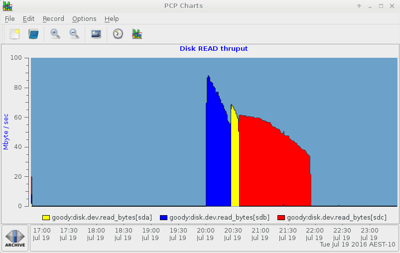
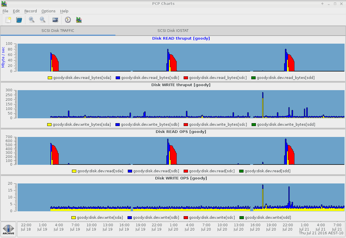
Note that the physvols in the vg volume group are linear, and we see traffic on sdb, then sda and then sdc become busy in turn, as our fake workload progresses in reading the three physvols comprising the vg-home volume group. If we instead had a stripe, we'd see simultaneous traffic on all three devices. We can visualize this more clearly with pmchart, e.g. :
Here's the pmchart IOSTAT view:
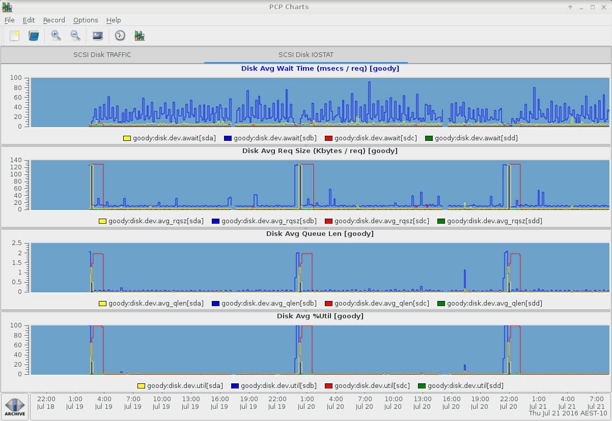
And here's the other pmchart tab showing the other iostat columns:
pmiostat - device selection and aggregation operators
A useful feature in pmiostat (version 3.11.2 or later) is the -R regex and -G sum|avg|min|max command line options. The regex selects a subset of the available devices (either sd devices, or device-mapper logical devices if the -x dm flag has been given). Only the selected devices will be reported, e.g.
# pmiostat -z -a myarchive -x t -t 10m -S'@Jul 19 19:45:00' -s 4 -P0 -R'sd[ab]$'
# Timestamp              Device       rrqm/s wrqm/s   r/s  w/s  rkB/s  wkB/s avgrq-sz avgqu-sz await r_await w_await %util
Tue Jul 19 19:55:00 2016 sda               0      0     0    1      0      3      2.0      0.0     5       0       5     1
Tue Jul 19 19:55:00 2016 sdb               0      0     0    1      1     10     10.8      0.0     8      12       7     1
Tue Jul 19 20:05:00 2016 sda               0      0     0    2      0      5      2.7      0.0     7       8       7     1
Tue Jul 19 20:05:00 2016 sdb               0      0   347    1  44030     12    126.4      1.1     3       3      78    50
Tue Jul 19 20:15:00 2016 sda               0      0     0    1      0      3      2.0      0.0     4      10       4     1
Tue Jul 19 20:15:00 2016 sdb               1      0   630    1  79970     10    126.7      2.0     3       3      66   100
Tue Jul 19 20:25:00 2016 sda               0      0     0    1      0      3      2.0      0.0     4       0       4     1
Tue Jul 19 20:25:00 2016 sdb               1      0   522    1  65988     12    126.2      2.1     4       4      77   100
Note the extended regex needs to be anchored with a trailing $ - otherwise we'll match sdaa, sdab, etc.
The -G flag allows aggregation of the statistics for the devices matching the regex supplied with the -R flag, or all devices by default if -R isn't supplied. As a practical example, we can check the HBTL scsi-id by querying the hinv.map.scsi metric, e.g. :
# pminfo -a myarchive -f hinv.map.scsi

hinv.map.scsi
    inst [0 or "scsi0:0:0:0 Direct-Access"] value "sda"
    inst [1 or "scsi1:0:0:0 Direct-Access"] value "sdb"
    inst [2 or "scsi2:0:0:0 Direct-Access"] value "sdc"
    inst [3 or "scsi3:0:0:0 Direct-Access"] value "sdd"
And let's say we want to sum the statistics for sda and sdb (e.g. because they might be alternate paths to the same target, or on the same PCI bus, whatever - and you're interested in summing that traffic) :
# pmiostat -z -a myarchive -x t -t 10m -S'@Jul 19 19:45:00' -s 4 -P0 -R'sd[ab]$' -Gsum
# Timestamp              Device       rrqm/s wrqm/s   r/s  w/s  rkB/s  wkB/s avgrq-sz avgqu-sz await r_await w_await %util
Tue Jul 19 19:55:00 2016 sum(sd[ab]$)      0      1     0    2      1     13     12.8      0.0    12      12      12     1
Tue Jul 19 20:05:00 2016 sum(sd[ab]$)      0      1   347    3  44030     17    129.1      1.1    10      11      85    51
Tue Jul 19 20:15:00 2016 sum(sd[ab]$)      1      0   630    2  79970     13    128.7      2.0     7      13      70   101
Tue Jul 19 20:25:00 2016 sum(sd[ab]$)      1      1   522    3  65988     15    128.2      2.1     8       4      80   101
Note that the device name column is now reported as the supplied regex pattern and that the %util column is always averaged, despite using the -Gsum flag.
dm-XX to logical volume name mapping
Internally, the kernel allocates device mapper devices dynamically and names them dm-XX. The mapping is dynamic and can change across reboots and a particular device mapper device name can be reused (if deleted and then a new device created). Kernel syslog messages usually report the dm-XX names, not the persistent logical device names used by LVM. So correlating the dynamic names used in kernel messages with LVM persistent names can be particularly arduous. Fortunately, PCP supports the hinv.map.dmname metric and we can use it in pmrep reports just like any other metric. Here is an example of the mapping :
# pminfo -a myarchive -f hinv.map.dmname

hinv.map.dmname
    inst [0 or "vg-swap"] value "dm-0"
    inst [1 or "vg-root"] value "dm-1"
    inst [3 or "vg-libvirt"] value "dm-2"
    inst [5 or "vg-home"] value "dm-3"
    inst [7 or "docker-253:1-4720837-pool"] value "dm-4"
    inst [273 or "docker-253:1-4720837-bd20b3551af42d2a0a6a3ed96cccea0fd59938b70e57a967937d642354e04859"] value "dm-5"
    inst [274 or "docker-253:1-4720837-b4aca4676507814fcbd56f81f3b68175e0d675d67bbbe371d16d1e5b7d95594e"] value "dm-6"
pmrep - other examples
When using pmrep, the hinv.map.dmname can be listed in it's own column, e.g.
# pmrep -a myarchive -X "Device Name" -z -g -t 10m -p -f%c -S'@19:45' -s 5 -i 'vg-.*' hinv.map.dmname disk.dm.read_bytes disk.dm.write_bytes
[ 1] - hinv.map.dmname["vg-swap"] - none
[ 1] - hinv.map.dmname["vg-root"] - none
[ 1] - hinv.map.dmname["vg-libvirt"] - none
[ 1] - hinv.map.dmname["vg-home"] - none
[ 2] - disk.dm.read_bytes["vg-swap"] - Kbyte/s
[ 2] - disk.dm.read_bytes["vg-root"] - Kbyte/s
[ 2] - disk.dm.read_bytes["vg-libvirt"] - Kbyte/s
[ 2] - disk.dm.read_bytes["vg-home"] - Kbyte/s
[ 3] - disk.dm.write_bytes["vg-swap"] - Kbyte/s
[ 3] - disk.dm.write_bytes["vg-root"] - Kbyte/s
[ 3] - disk.dm.write_bytes["vg-libvirt"] - Kbyte/s
[ 3] - disk.dm.write_bytes["vg-home"] - Kbyte/s

                                              1         2         3
Mon Jul 18 19:45:00 2016      vg-swap      dm-0       N/A       N/A
Mon Jul 18 19:45:00 2016      vg-root      dm-1       N/A       N/A
Mon Jul 18 19:45:00 2016   vg-libvirt      dm-2       N/A       N/A
Mon Jul 18 19:45:00 2016      vg-home      dm-3       N/A       N/A
Mon Jul 18 19:55:00 2016      vg-swap      dm-0     0.187     0.000
Mon Jul 18 19:55:00 2016      vg-root      dm-1     0.000     9.617
Mon Jul 18 19:55:00 2016   vg-libvirt      dm-2     0.000     2.703
Mon Jul 18 19:55:00 2016      vg-home      dm-3     0.000     0.000
Mon Jul 18 20:05:00 2016      vg-swap      dm-0     0.500     0.000
Mon Jul 18 20:05:00 2016      vg-root      dm-1     5.037    11.875
Mon Jul 18 20:05:00 2016   vg-libvirt      dm-2     0.020     5.337
Mon Jul 18 20:05:00 2016      vg-home      dm-3  44082.53     0.000
Mon Jul 18 20:15:00 2016      vg-swap      dm-0     0.240     0.000
Mon Jul 18 20:15:00 2016      vg-root      dm-1     8.888     9.778
Mon Jul 18 20:15:00 2016   vg-libvirt      dm-2     0.007     3.007
Mon Jul 18 20:15:00 2016      vg-home      dm-3  79842.49     0.000
Mon Jul 18 20:25:00 2016      vg-swap      dm-0     0.190     0.000
Mon Jul 18 20:25:00 2016      vg-root      dm-1    31.063    11.827
Mon Jul 18 20:25:00 2016   vg-libvirt      dm-2     0.013     3.093
Mon Jul 18 20:25:00 2016      vg-home      dm-3  65993.43     0.000
Note above we've used the -X flag with the heading "Device Name" to transpose the report (swap columns with rows). We've used the -g flag to list the details of each column heading before the main report. We've specified the -z flag to timestamps are in the timezone of the archive and -f%c to specify we want full ctime(3) timestamps rather than the default abbreviated version. We've also used the -i flag to restrict the report to only instances matching vg-.*. And finally, we've included both the dm-X and persistent LV names as separate columns in the report.
Another really handy feature of pmrep is pre-configured report columns. These are defined in pmrep.conf (usually found in /etc/pcp/pmrep/pmrep.conf). For example, the pre-configured :vmstat report can be combined with an additional column to show total disk traffic as follows:
# pmrep -a myarchive -z -t 10m -p -S'@19:45' -s 5 disk.all.total_bytes :vmstat
         d.a.total_bytes   r   b    swpd     free    buff   cache    si    so     bi     bo    in     cs  us  sy  id  wa  st
19:45:00             N/A   1   0 1460764  1261236 1968296 3504052   N/A   N/A    N/A    N/A   N/A    N/A N/A N/A N/A N/A N/A
19:55:00              13   1   0 1460664  1255956 1969544 3507748     0     0      0     12   283    387   0   0  99   0   0
20:05:00           44105   2   0 1460448    51976 6138692  540784     0     0  44088     18   848   1260   0   1  90   7   0
20:15:00           79864   1   1 1460300    51196 6229432  451360     0     0  79851     12  1336   1901   0   2  78  18   0
20:25:00           66040   1   2 1460180    50864 6226808  453452     0     0  66024     15  1333   1656   0   2  74  22   0
Notice the :vmstat specification is prefixed with :. There are many pre-defined report configuration entries in pmrep.conf - take a look. You can also define your own, as described in the pmrep(1) man page.
Non-interpolated mode
By default, all PCP monitoring tools use an interpolation mechanism, to allow the reporting interval to differ from the underlying native sampling interval. For details on how this works, see PCPIntro(1). Sometimes we do not want to use interpolation, e.g. when correlating blktrace(1) data with pmiostat data, we will need to match timestamps exactly. To disable interpolation, use the -u flag with pmrep or pmiostat.
Note that the -u flag is incompatible with the -t flag - when not using interpolation the sampling interval cannot be changed, it's always the same as the underlying sampling interval that the data was originally recorded with.
Tools for reporting per-process I/O
The pcp-atop(1) command can be used to examine per-process I/O statistics, and a wealth of other system level performance data. Like all PCP tools, pcp-atop can replay archives, provided the appropriate pmlogconf settings have been enabled - see above. For per-process I/O analysis, use the pcp -a ARCHIVE atop -d flag. You probably also want to specify a fairly long sampling interval because atop runs fairly slowly on large archives, especially when proc data is present. There are a large number of options. For process I/O, the -d flag is most useful.
# pcp atop --help
Usage: pcp-atop [-flags] [interval [samples]]
        or
Usage: pcp-atop -w  file  [-S] [-a] [interval [samples]]
       pcp-atop -r  file  [-b hh:mm] [-e hh:mm] [-flags]

    generic flags:
      -a  show or log all processes (i.s.o. active processes only)
      -R  calculate proportional set size (PSS) per process
      -P  generate parseable output for specified label(s)
      -L  alternate line length (default 80) in case of non-screen output
      -f  show fixed number of lines with system statistics
      -F  suppress sorting of system resources
      -G  suppress exited processes in output
      -l  show limited number of lines for certain resources
      -y  show individual threads
      -1  show average-per-second i.s.o. total values

      -x  no colors in case of high occupation
      -g  show general process-info (default)
      -m  show memory-related process-info
      -d  show disk-related process-info
      -n  show network-related process-info
      -s  show scheduling-related process-info
      -v  show various process-info (ppid, user/group, date/time)
      -c  show command line per process
      -o  show own defined process-info
      -u  show cumulated process-info per user
      -p  show cumulated process-info per program (i.e. same name)

      -C  sort processes in order of cpu-consumption (default)
      -M  sort processes in order of memory-consumption
      -D  sort processes in order of disk-activity
      -N  sort processes in order of network-activity
      -A  sort processes in order of most active resource (auto mode)

    specific flags for raw logfiles:
      -w  write raw data to PCP archive folio
      -r  read  raw data from PCP archive folio
      -S  finish pcp-atop automatically before midnight (i.s.o. #samples)
      -b  begin showing data from specified time
      -e  finish showing data after specified time

    interval: number of seconds   (minimum 0)
    samples:  number of intervals (minimum 1)
Finding blocked processes
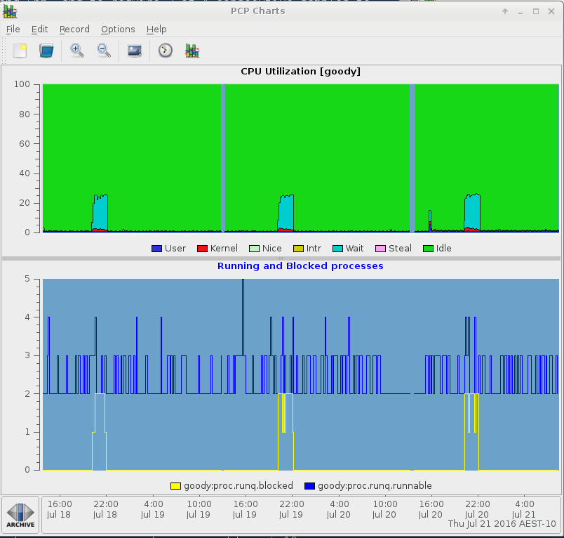
One common task in I/O performance analysis involves blocked tasks, i.e. processes in 'D' state or UN uninterruptible sleep. It's easy to check this with pmchart by plotting the proc.runq.runnable and proc.runq.blocked process counts, e.g.
# pmchart -z -a myarchive -t 10m -O-0 -s 400 -v 400 -geometry 800x450 -c CPU
To monitor specific processes, you can also use the pmrep and pcp-pidstat tools, and others. The pcp-pidstat tool is currently being developed with additional features to detect and monitor blocked processes.
References
Knowledge Base Articles and Solutions
- Index of Performance Co-Pilot (PCP) articles, solutions, tutorials and white papers
- PCP Data Sheet
- How do I install Performance Co-Pilot (PCP) on my RHEL server to capture performance logs
- What are all the Performance Co-Pilot (PCP) RPM packages in RHEL?
- How to use Performance Co-Pilot
- How do I gather performance data logs to upload to my support case using Performance Co-Pilot (PCP)
- How can I merge multiple PCP archives into one for a system level performance analysis covering multiple days or weeks
- How can I use Performance Co-Pilot (PCP) to capture a "once-off" performance data archive log for a specific interval of time
- How is Performance Co-Pilot (PCP) designed and structured?
- What are the typical Performance Co-Pilot (PCP) deployment strategies?
- How can I customize the Performance Co-Pilot logging configuration
- How can I change the default logging interval used by Performance Co-Pilot (PCP)?
- Are Red Hat planning to include PCP (Performance Co-Pilot) in RHEL?
- How do I configure a firewall on a RHEL server to allow remote monitoring with Performance Co-Pilot (PCP)?
- How does Performance Co-Pilot (PCP) compare with sysstat
- Side-by-side comparison of PCP tools with legacy tools
- How to use a non-default PMDA with PCP?
- pmiostat fails to replay a PCP archive log created on a RHEL6 system
- Overview of Additional Performance Tuning Utilities in Red Hat Enterprise Linux 7
- Interactive web interface for Performance Co-Pilot
- How can I convert a collectl archive into a Performance Co-Pilot (PCP) archive?
Comments