
OpenShift AI tutorial - Fraud detection example
Use OpenShift AI to train an example model in a Jupyter notebook, deploy the model, and refine the model by using automated pipelines
Abstract
Chapter 1. Introduction
Welcome!
In this tutorial, you learn how to incorporate data science and artificial intelligence and machine learning (AI/ML) into an OpenShift development workflow.
You will use an example fraud detection model to complete the following tasks:
- Explore a pre-trained fraud detection model by using a Jupyter notebook.
- Deploy the model by using OpenShift AI model serving.
- Refine and train the model by using automated pipelines.
And you do not have to install anything on your own computer, thanks to Red Hat OpenShift AI.
1.1. About the example fraud detection model
The example fraud detection model monitors credit card transactions for potential fraudulent activity. It analyzes the following credit card transaction details:
- The geographical distance from the previous credit card transaction.
- The price of the current transaction, compared to the median price of all the user’s transactions.
- Whether the user completed the transaction by using the hardware chip in the credit card, entered a PIN number, or for an online purchase.
Based on this data, the model outputs the likelihood of the transaction being fraudulent.
1.2. Before you begin
If you don’t already have an instance of Red Hat OpenShift AI, see the Red Hat OpenShift AI page on the Red Hat Developer website for information on setting up your environment. There, you can create an account and access the free OpenShift AI Sandbox or you can learn how to install OpenShift AI on your own OpenShift cluster.
If your cluster uses self-signed certificates, before you begin the tutorial, your OpenShift AI administrator must add self-signed certificates for OpenShift AI as described in Working with certificates.
If you’re ready, start the tutorial!
Chapter 2. Setting up a project and storage
2.1. Navigating to the OpenShift AI dashboard
Procedure
After you log in to the OpenShift console, access the OpenShift AI dashboard by clicking the application launcher icon on the header.
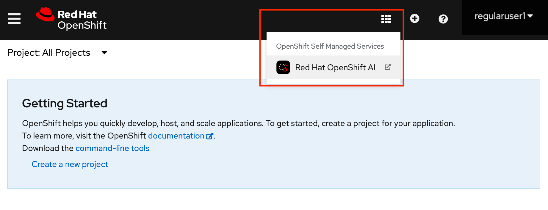
When prompted, log in to the OpenShift AI dashboard by using your OpenShift credentials. OpenShift AI uses the same credentials as OpenShift for the dashboard, notebooks, and all other components.
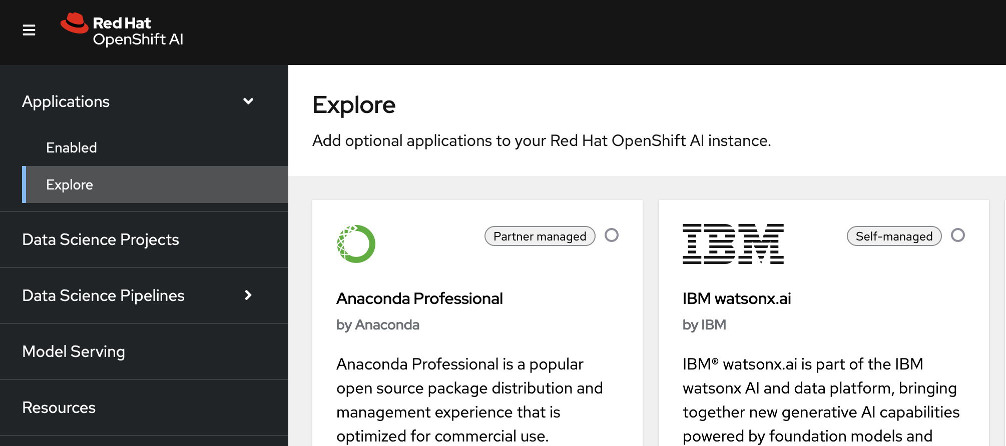
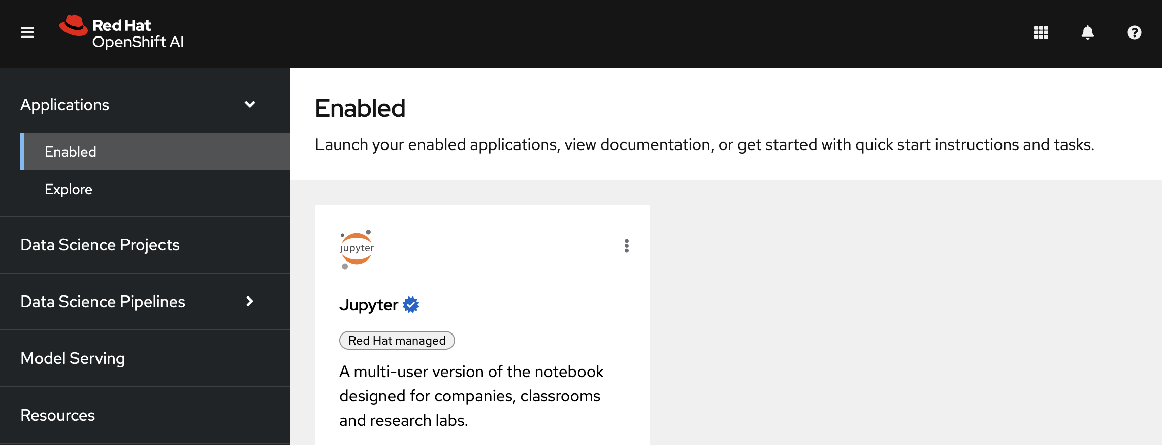
The OpenShift AI dashboard shows the status of any installed and enabled applications.
Optionally, click Explore to view other available application integrations.
Note: You can navigate back to the OpenShift console in a similar fashion. Click the application launcher to access the OpenShift console.
For now, stay in the OpenShift AI dashboard.
Next step
2.2. Setting up your data science project
Before you begin, make sure that you are logged in to Red Hat OpenShift AI and that you can see the dashboard:
Note that you can start a Jupyter notebook from here, but it would be a one-off notebook run in isolation. To implement a data science workflow, you must create a data science project. Projects allow you and your team to organize and collaborate on resources within separated namespaces. From a project you can create multiple workbenches, each with their own Jupyter notebook environment, and each with their own data connections and cluster storage. In addition, the workbenches can share models and data with pipelines and model servers.
Procedure
On the navigation menu, select Data Science Projects. This page lists any existing projects that you have access to. From this page, you can select an existing project (if any) or create a new one.
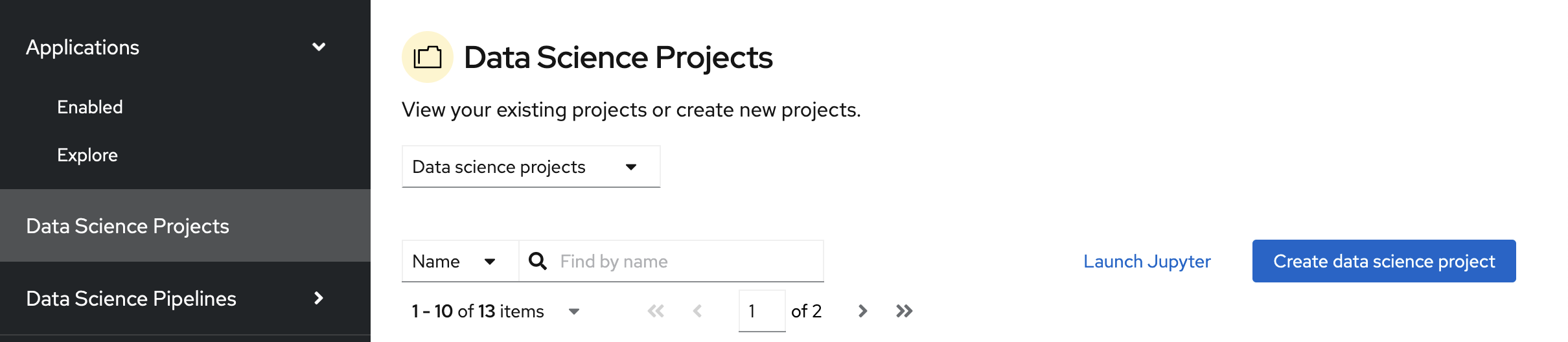
If you already have an active project that you want to use, select it now and skip ahead to the next section, Storing data with data connections. Otherwise, continue to the next step.
- Click Create data science project.
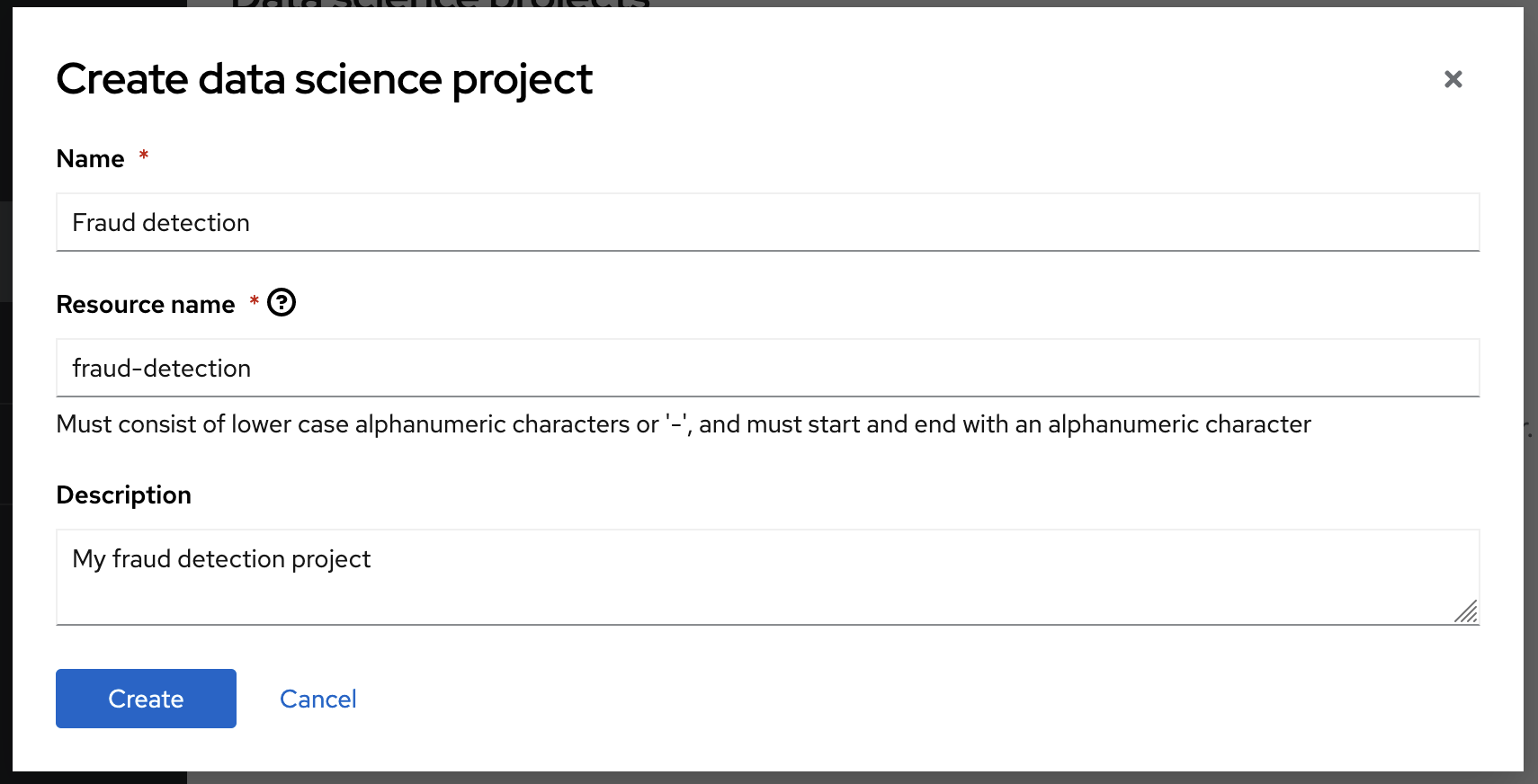
Enter a display name and description. Based on the display name, a resource name is automatically generated, but you can change it if you prefer.
Verification
You can now see its initial state. Individual tabs provide more information about the project components and project access permissions:
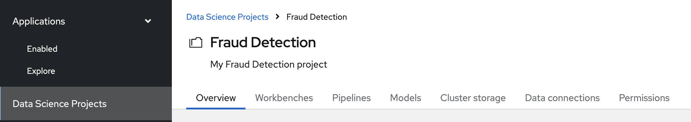
- Workbenches are instances of your development and experimentation environment. They typically contain IDEs, such as JupyterLab, RStudio, and Visual Studio Code.
- Pipelines contain the data science pipelines that are executed within the project.
- Models allow you to quickly serve a trained model for real-time inference. You can have multiple model servers per data science project. One model server can host multiple models.
- Cluster storage is a persistent volume that retains the files and data you’re working on within a workbench. A workbench has access to one or more cluster storage instances.
- Data connections contain configuration parameters that are required to connect to a data source, such as an S3 object bucket.
- Permissions define which users and groups can access the project.
Next step
2.3. Storing data with data connections
For this tutorial, you need two S3-compatible object storage buckets, such as Ceph, Minio, or AWS S3:
- My Storage - Use this bucket for storing your models and data. You can reuse this bucket and its connection for your notebooks and model servers.
- Pipelines Artifacts - Use this bucket as storage for your pipeline artifacts. A pipeline artifacts bucket is required when you create a pipeline server. For this tutorial, create this bucket to separate it from the first storage bucket for clarity.
You can use your own storage buckets or run a provided script that creates local Minio storage buckets for you.
Also, you must create a data connection to each storage bucket. A data connection is a resource that contains the configuration parameters needed to connect to an object storage bucket.
You have two options for this tutorial, depending on whether you want to use your own storage buckets or use a script to create local Minio storage buckets:
- If you want to use your own S3-compatible object storage buckets, create data connections to them as described in Creating data connections to your own S3-compatible object storage.
- If you want to run a script that installs local Minio storage buckets and creates data connections to them, for the purposes of this tutorial, follow the steps in Running a script to install local object storage buckets and create data connections.
2.3.1. Creating data connections to your own S3-compatible object storage
If you do not have your own s3-compatible storage, or if you want to use a disposable local Minio instance instead, skip this section and follow the steps in Running a script to install local object storage buckets and create data connections.
Prerequisite
To create data connections to your existing S3-compatible storage buckets, you need the following credential information for the storage buckets:
- Endpoint URL
- Access key
- Secret key
- Region
- Bucket name
If you don’t have this information, contact your storage administrator.
Procedures
Create data connections to your two storage buckets.
Create a data connection for saving your data and models
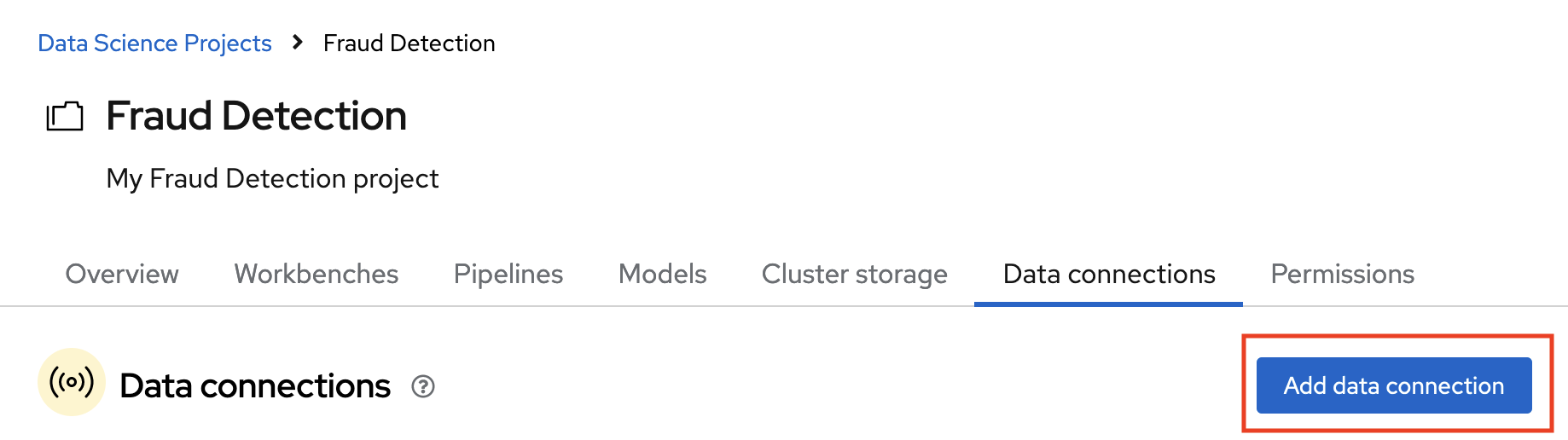
- In the OpenShift AI dashboard, navigate to the page for your data science project.
Click the Data connections tab, and then click Add data connection.
Fill out the Add data connection form and name your connection My Storage. This connection is for saving your personal work, including data and models.
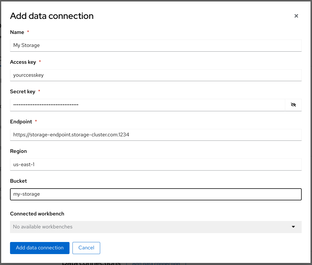
- Click Add data connection.
Create a data connection for saving pipeline artifacts
If you do not intend to complete the pipelines section of the tutorial, you can skip this step.
- Click Add data connection.
Fill out the form and name your connection Pipeline Artifacts.
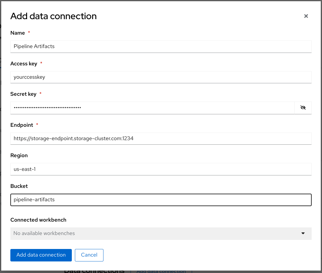
- Click Add data connection.
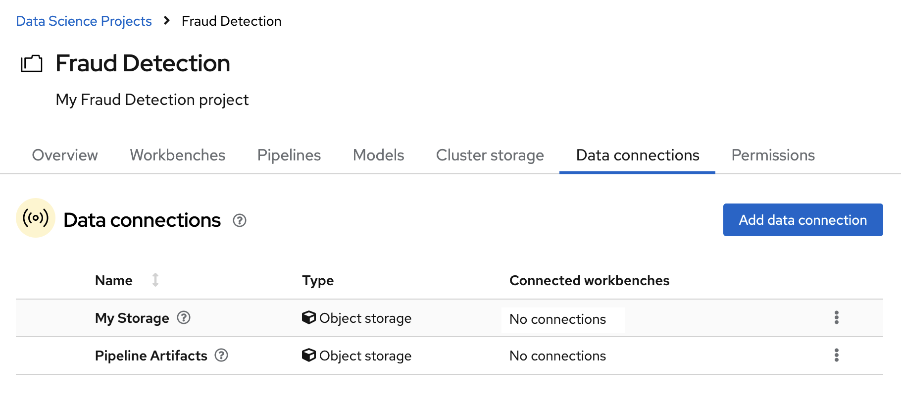
Verification
In the Data connections tab for the project, check to see that your data connections are listed.
Next steps
- Configure a pipeline server as described in Enabling data science pipelines
- Create a workbench and select a notebook image as described in Creating a workbench
2.3.2. Running a script to install local object storage buckets and create data connections
For convenience, run a script (provided in the following procedure) that automatically completes these tasks:
- Creates a Minio instance in your project.
- Creates two storage buckets in that Minio instance.
- Generates a random user id and password for your Minio instance.
- Creates two data connections in your project, one for each bucket and both using the same credentials.
- Installs required network policies for service mesh functionality.
The script is based on a guide for deploying Minio.
The Minio-based Object Storage that the script creates is not meant for production usage.
If you want to connect to your own storage, see Creating data connections to your own S3-compatible object storage.
Prerequisite
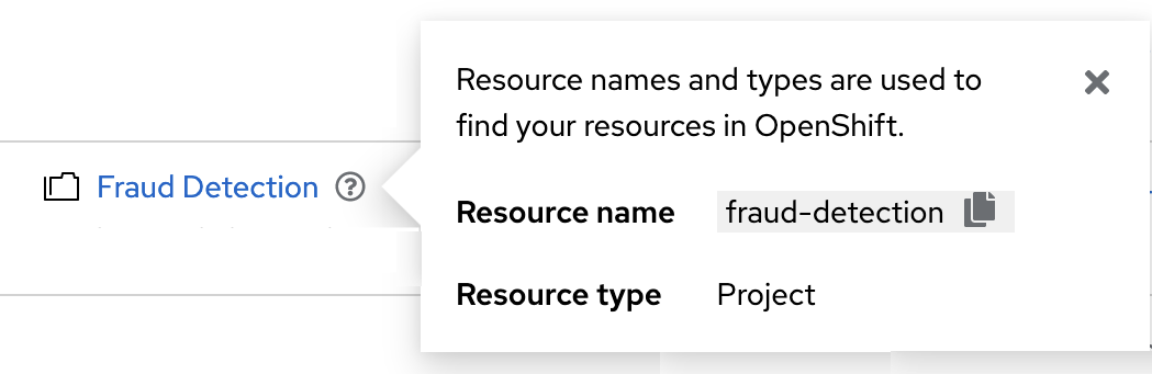
You must know the OpenShift resource name for your data science project so that you run the provided script in the correct project. To get the project’s resource name:
In the OpenShift AI dashboard, select Data Science Projects and then click the ? icon next to the project name. A text box appears with information about the project, including its resource name:
The following procedure describes how to run the script from the OpenShift console. If you are knowledgeable in OpenShift and can access the cluster from the command line, instead of following the steps in this procedure, you can use the following command to run the script:
oc apply -n <your-project-name/> -f https://github.com/rh-aiservices-bu/fraud-detection/raw/main/setup/setup-s3.yaml
Procedure
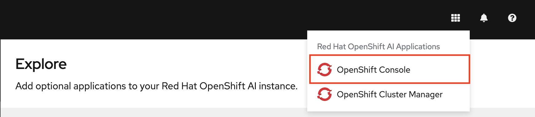
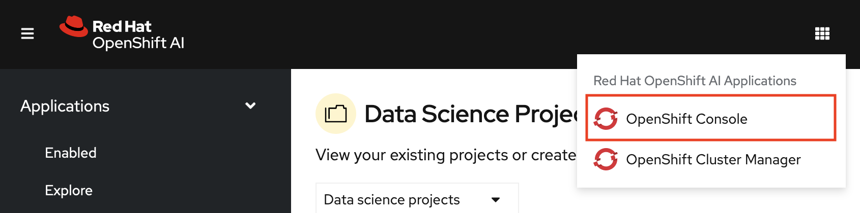
In the OpenShift AI dashboard, click the application launcher icon and then select the OpenShift Console option.
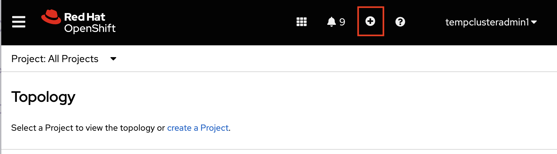
In the OpenShift console, click + in the top navigation bar.
Select your project from the list of projects.
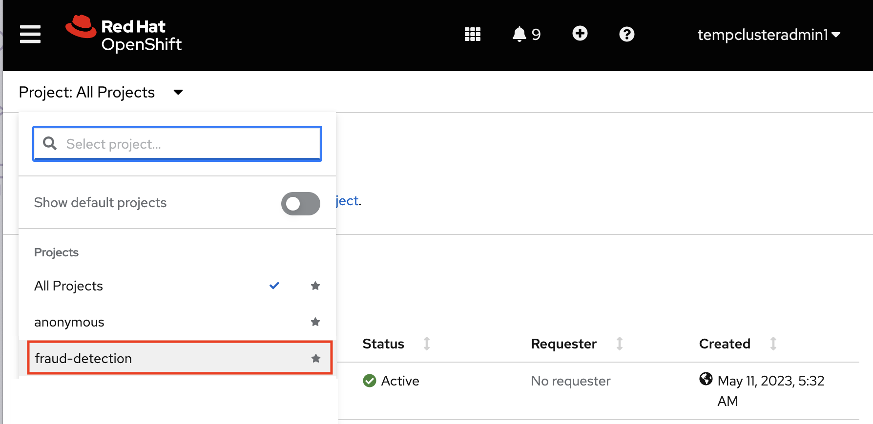
Verify that you selected the correct project.
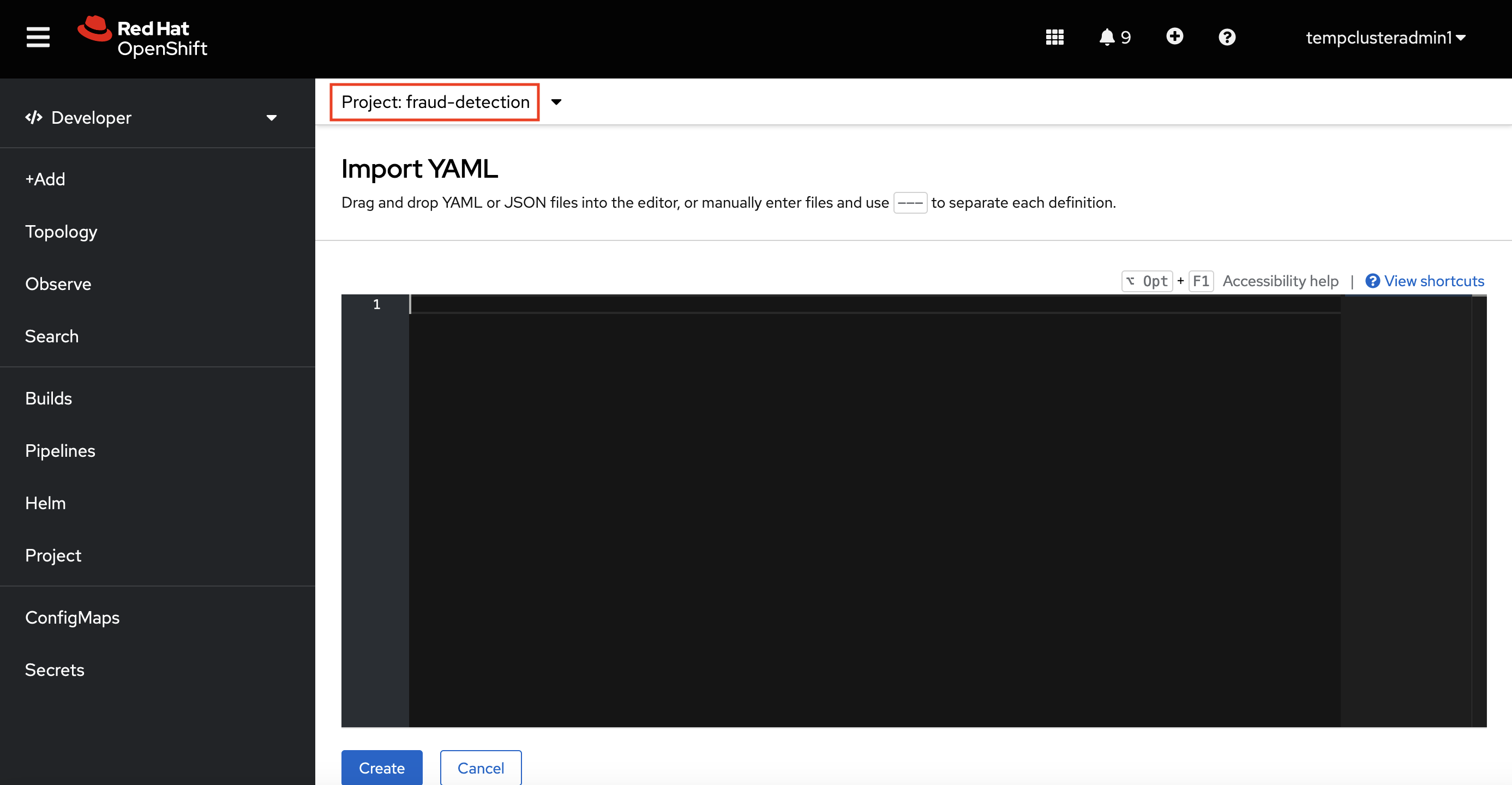
Copy the following code and paste it into the Import YAML editor.
Note: This code gets and applies the
setup-s3-no-sa.yamlfile.--- apiVersion: v1 kind: ServiceAccount metadata: name: demo-setup --- apiVersion: rbac.authorization.k8s.io/v1 kind: RoleBinding metadata: name: demo-setup-edit roleRef: apiGroup: rbac.authorization.k8s.io kind: ClusterRole name: edit subjects: - kind: ServiceAccount name: demo-setup --- apiVersion: batch/v1 kind: Job metadata: name: create-s3-storage spec: selector: {} template: spec: containers: - args: - -ec - |- echo -n 'Setting up Minio instance and data connections' oc apply -f https://github.com/rh-aiservices-bu/fraud-detection/raw/main/setup/setup-s3-no-sa.yaml command: - /bin/bash image: image-registry.openshift-image-registry.svc:5000/openshift/tools:latest imagePullPolicy: IfNotPresent name: create-s3-storage restartPolicy: Never serviceAccount: demo-setup serviceAccountName: demo-setup- Click Create.
Verification
You should see a "Resources successfully created" message and the following resources listed:
-
demo-setup -
demo-setup-edit -
create s3-storage
Next steps
- Configure a pipeline server as described in Enabling data science pipelines
- Create a workbench and select a notebook image as described in Creating a workbench
2.4. Enabling data science pipelines
If you do not intend to complete the pipelines section of the workshop you can skip this step and move on to the next section, Create a Workbench.
In this section, you prepare your tutorial environment so that you can use data science pipelines.
In this tutorial, you implement an example pipeline by using the JupyterLab Elyra extension. With Elyra, you can create a visual end-to-end pipeline workflow that can be executed in OpenShift AI.
Prerequisite
- You have installed local object storage buckets and created data connections, as described in Storing data with data connections.
Procedure
- In the OpenShift AI dashboard, click Data Science Projects and then select Fraud Detection.
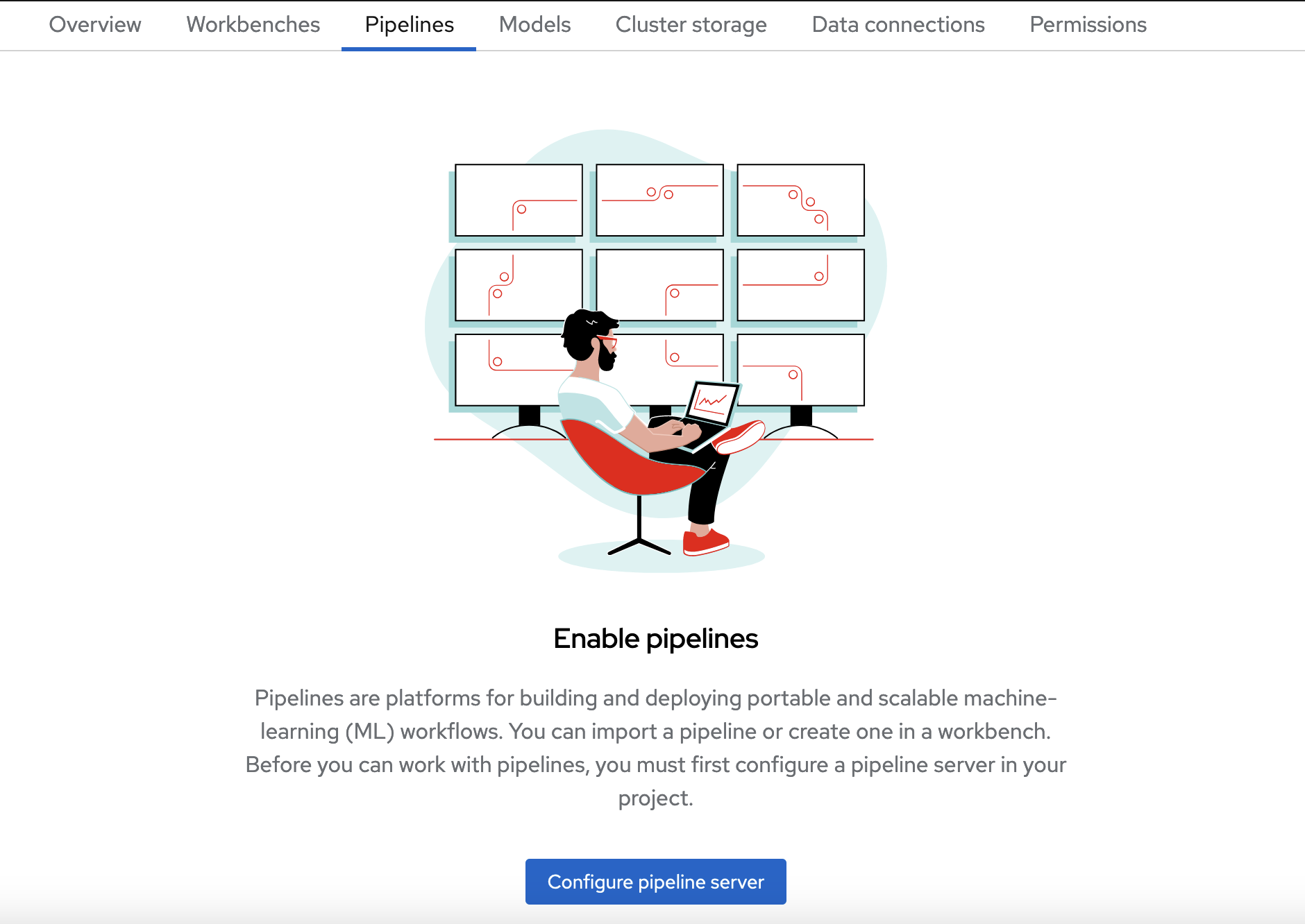
- Click the Pipelines tab.
Click Configure pipeline server.
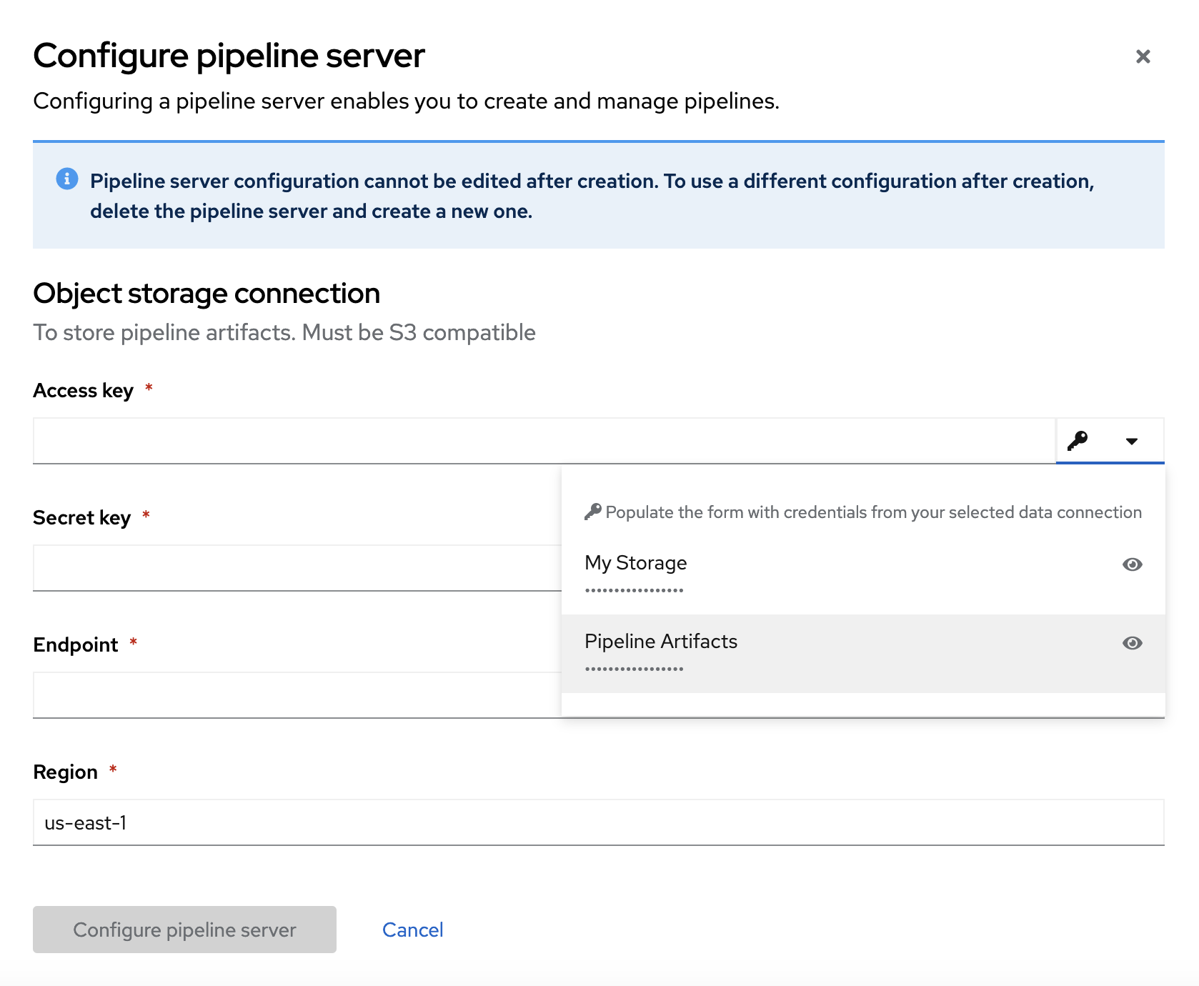
In the Configure pipeline server form, in the Access key field next to the key icon, click the dropdown menu and then click Pipeline Artifacts to populate the Configure pipeline server form with credentials for the data connection.
- Leave the database configuration as the default.
- Click Configure pipeline server.
- Wait until the spinner disappears and No pipelines yet is displayed.
You must wait until the pipeline configuration is complete before you continue and create your workbench. If you create your workbench before the pipeline server is ready, your workbench will not be able to submit pipelines to it.
Verification
- Navigate to the Pipelines tab for the project.
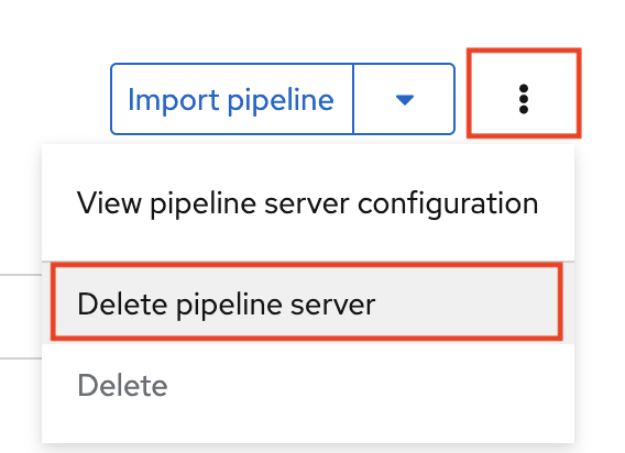
Next to Import pipeline, click the action menu (⋮) and then select View pipeline server configuration.
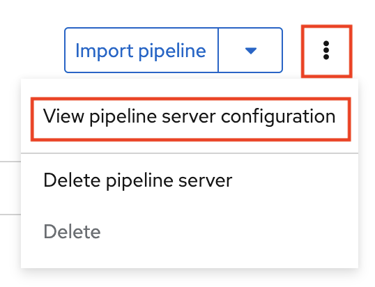
An information box opens and displays the object storage connection information for the pipeline server.
If you have waited more than 5 minutes, and the pipeline server configuration does not complete, you can try to delete the pipeline server and create it again.
You can also ask your OpenShift AI administrator to verify that self-signed certificates are added to your cluster as described in Working with certificates.
Chapter 3. Creating a workbench and a notebook
3.1. Creating a workbench and selecting a notebook image
A workbench is an instance of your development and experimentation environment. Within a workbench you can select a notebook image for your data science work.
Prerequisites
-
You created a
My Storagedata connection as described in Storing data with data connections. - You configured a pipeline server as described in Enabling data science pipelines.
Procedure
- Navigate to the project detail page for the data science project that you created in Setting up your data science project.
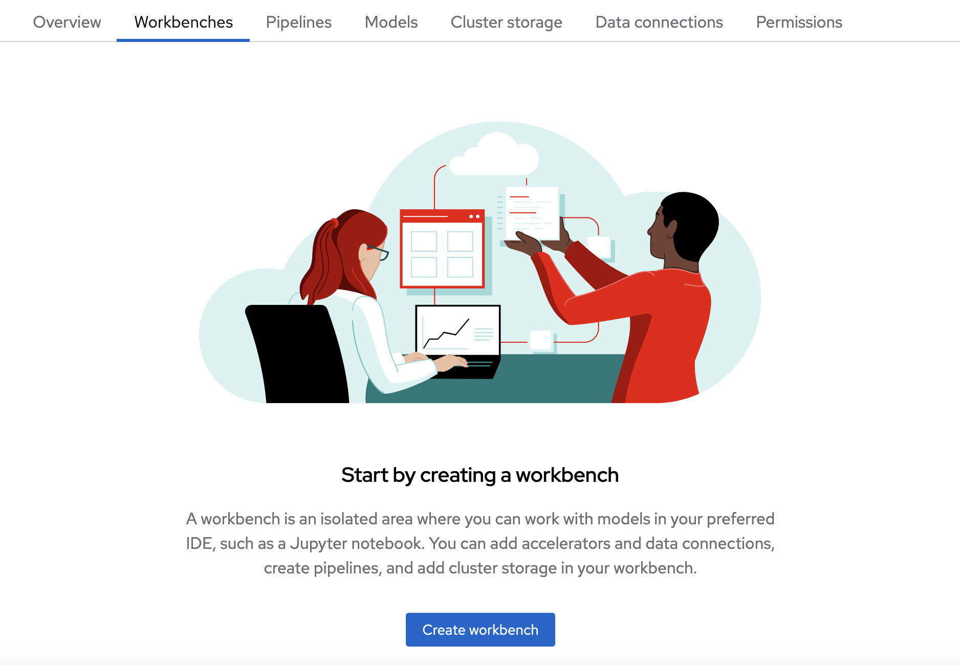
Click the Workbenches tab, and then click the Create workbench button.
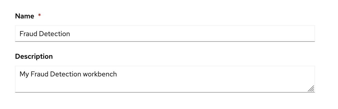
Fill out the name and description.
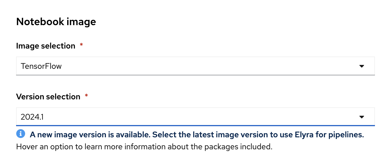
Red Hat provides several supported notebook images. In the Notebook image section, you can choose one of these images or any custom images that an administrator has set up for you. The Tensorflow image has the libraries needed for this tutorial.
Select the latest Tensorflow image.
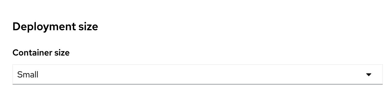
Choose a small deployment.
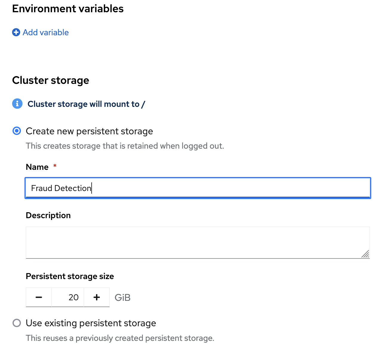
Leave the default environment variables and storage options.
Under Data connections, select Use existing data connection and select
My Storage(the object storage that you configured previously) from the list.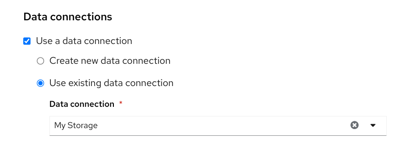
Click the Create workbench button.

Verification
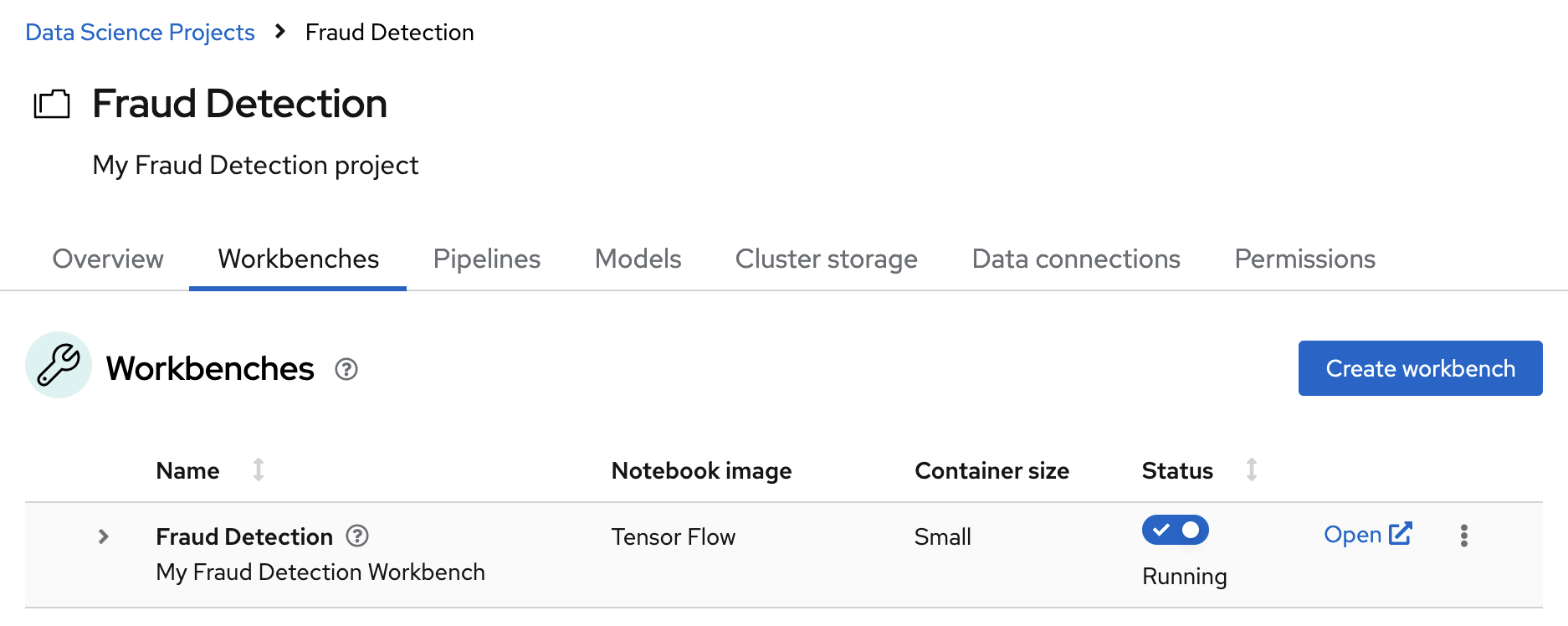
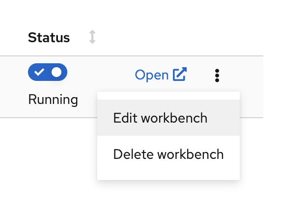
In the Workbenches tab for the project, the status of the workbench changes from Starting to Running.
If you made a mistake, you can edit the workbench to make changes.
3.2. Importing the tutorial files into the Jupyter environment
The Jupyter environment is a web-based environment, but everything you do inside it happens on Red Hat OpenShift AI and is powered by the OpenShift cluster. This means that, without having to install and maintain anything on your own computer, and without disposing of valuable local resources such as CPU, GPU and RAM, you can conduct your data science work in this powerful and stable managed environment.
Prerequisite
You created a workbench, as described in Creating a workbench and selecting a Notebook image.
Procedure
Click the Open link next to your workbench. If prompted, log in and allow the Notebook to authorize your user.

Your Jupyter environment window opens.
This file-browser window shows the files and folders that are saved inside your own personal space in OpenShift AI.
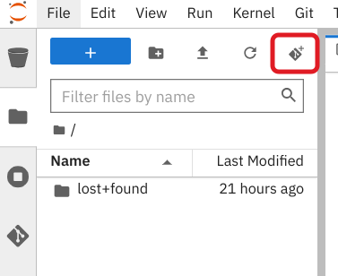
Bring the content of this tutorial inside your Jupyter environment:
On the toolbar, click the Git Clone icon:
Enter the following tutorial Git https URL:
https://github.com/rh-aiservices-bu/fraud-detection.git
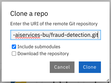
- Check the Include submodules option.
- Click Clone.
Verification
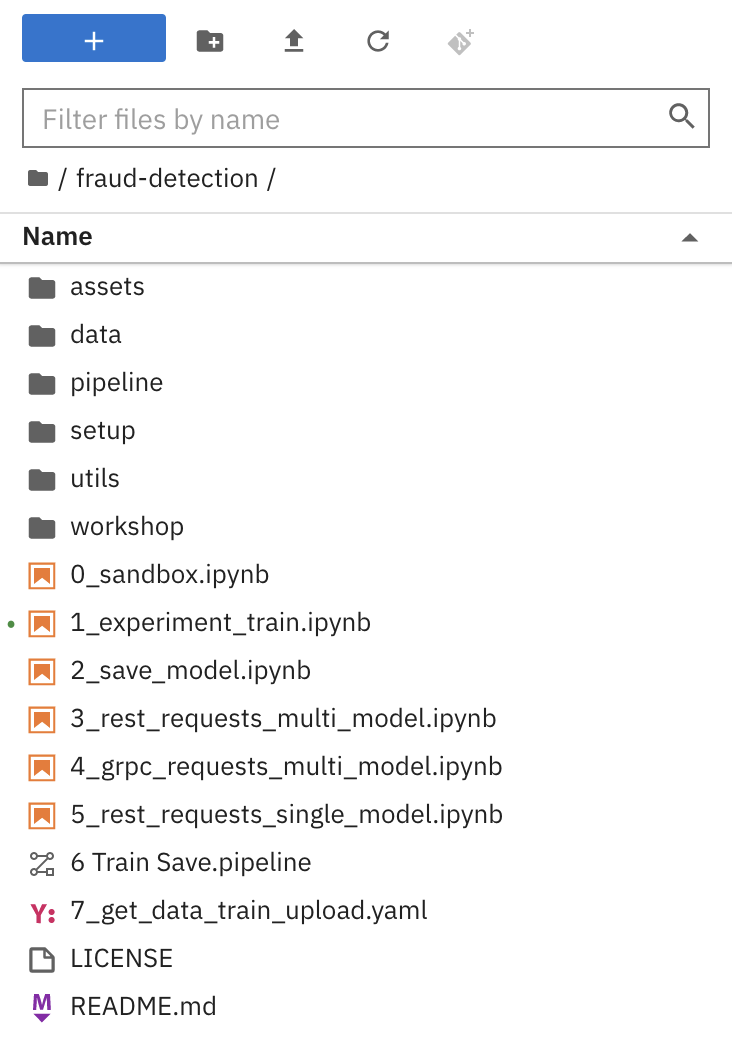
Double-click the newly-created folder, fraud-detection:
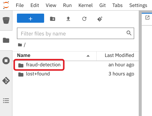
In the file browser, you should see the notebooks that you cloned from Git.
Next step
or
3.3. Running code in a notebook
If you’re already at ease with Jupyter, you can skip to the next section.
A notebook is an environment where you have cells that can display formatted text or code.
This is an empty cell:

This is a cell with some code:
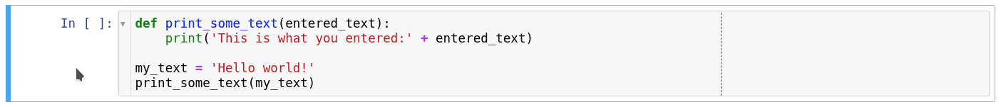
Code cells contain Python code that you can run interactively. You can modify the code and then run it. The code does not run on your computer or in the browser, but directly in the environment that you are connected to, Red Hat OpenShift AI in our case.
You can run a code cell from the notebook interface or from the keyboard:
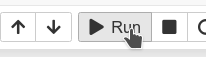
From the user interface: Select the cell (by clicking inside the cell or to the left side of the cell) and then click Run from the toolbar.
-
From the keyboard: Press
CTRL+ENTERto run a cell or pressSHIFT+ENTERto run the cell and automatically select the next one.
After you run a cell, you can see the result of its code as well as information about when the cell was run, as shown in this example:
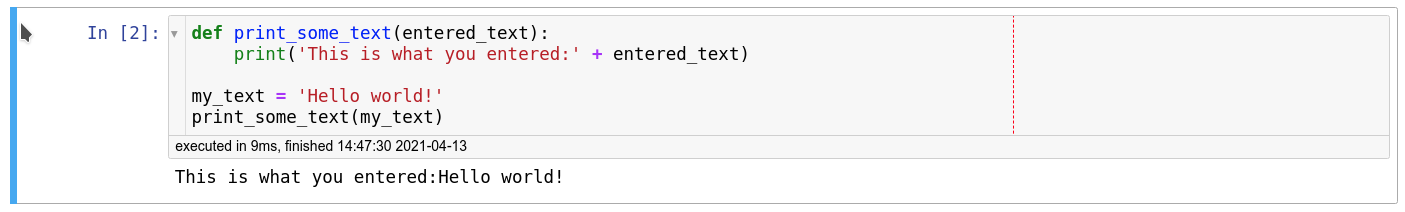
When you save a notebook, the code and the results are saved. You can reopen the notebook to look at the results without having to run the program again, while still having access to the code.
Notebooks are so named because they are like a physical notebook: you can take notes about your experiments (which you will do), along with the code itself, including any parameters that you set. You can see the output of the experiment inline (this is the result from a cell after it’s run), along with all the notes that you want to take (to do that, from the menu switch the cell type from Code to Markdown).
3.3.1. Try it
Now that you know the basics, give it a try!
Prerequisite
- You have imported the tutorial files into your Jupyter environment as described in Importing the tutorial files into the Jupyter environment.
Procedure
In your Jupyter environment, locate the
0_sandbox.ipynbfile and double-click it to launch the notebook. The notebook opens in a new tab in the content section of the environment.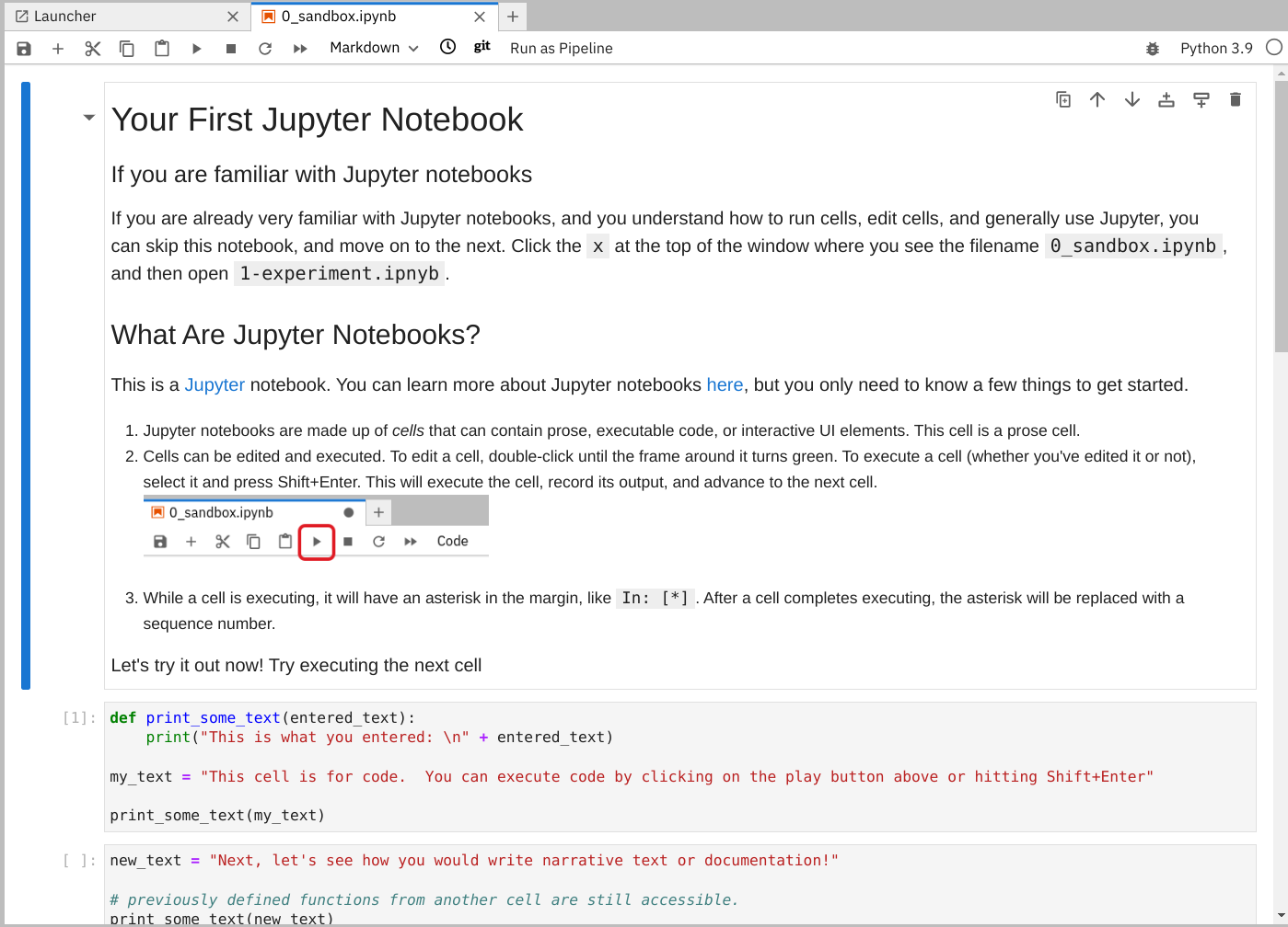
Experiment by, for example, running the existing cells, adding more cells and creating functions.
You can do what you want - it’s your environment and there is no risk of breaking anything or impacting other users. This environment isolation is also a great advantage brought by OpenShift AI.
Optionally, create a new notebook in which the code cells are run by using a Python 3 kernel:
Create a new notebook by either selecting File →New →Notebook or by clicking the Python 3 tile in the Notebook section of the launcher window:
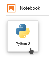
You can use different kernels, with different languages or versions, to run in your notebook.
Additional resource
To learn more about notebooks, go to the Jupyter site.
Next step
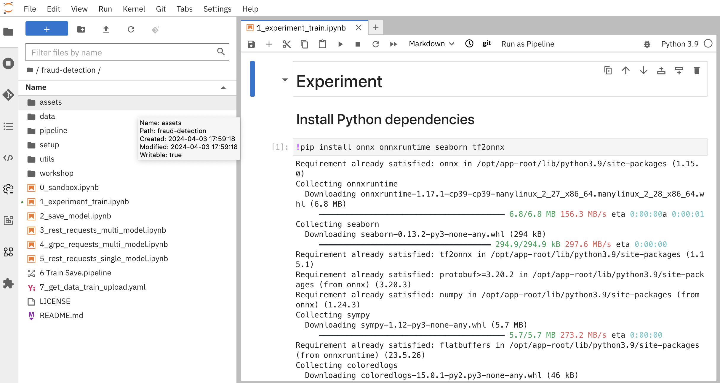
3.4. Training a model
Now that you know how the Jupyter notebook environment works, the real work can begin!
In your notebook environment, open the 1_experiment_train.ipynb file and follow the instructions directly in the notebook. The instructions guide you through some simple data exploration, experimentation, and model training tasks.
Next step
Chapter 4. Deploying and testing a model
4.1. Preparing a model for deployment
After you train a model, you can deploy it by using the OpenShift AI model serving capabilities.
To prepare a model for deployment, you must move the model from your workbench to your S3-compatible object storage. You use the data connection that you created in the Storing data with data connections section and upload the model from a notebook. You also convert the model to the portable ONNX format. ONNX allows you to transfer models between frameworks with minimal preparation and without the need for rewriting the models.
Prerequisites
You created the data connection
My Storage.You added the
My Storagedata connection to your workbench.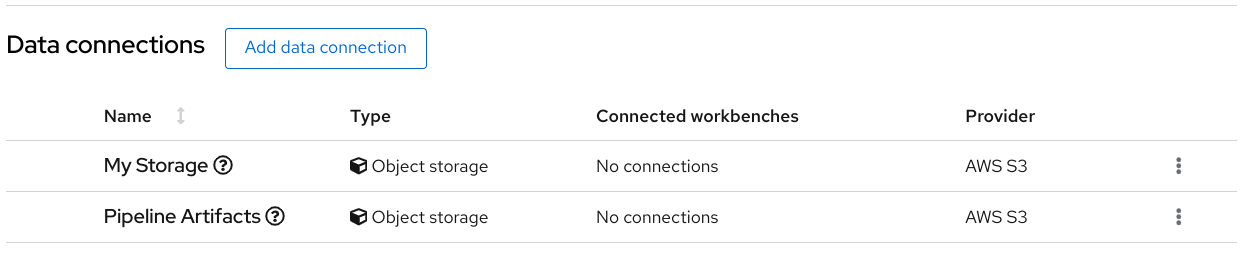
Procedure
-
In your Jupyter environment, open the
2_save_model.ipynbfile. - Follow the instructions in the notebook to make the model accessible in storage and save it in the portable ONNX format.
Verification
When you have completed the notebook instructions, the models/fraud/1/model.onnx file is in your object storage and it is ready for your model server to use.
Next step
4.2. Deploying a model
Now that the model is accessible in storage and saved in the portable ONNX format, you can use an OpenShift AI model server to deploy it as an API.
OpenShift AI offers two options for model serving:
- Single-model serving - Each model in the project is deployed on its own model server. This platform is suitable for large models or models that need dedicated resources.
- Multi-model serving - All models in the project are deployed on the same model server. This platform is suitable for sharing resources amongst deployed models.
Note: For each project, you can specify only one model serving platform. If you want to change to the other model serving platform, you must create a new project.
For this tutorial, since you are only deploying only one model, you can select either serving type. The steps for deploying the fraud detection model depend on the type of model serving platform you select:
4.2.1. Deploying a model on a single-model server
OpenShift AI single-model servers host only one model. You create a new model server and deploy your model to it.
Prerequiste
-
A user with
adminprivileges has enabled the single-model serving platform on your OpenShift cluster.
Procedure
In the OpenShift AI dashboard, navigate to the project details page and click the Models tab.
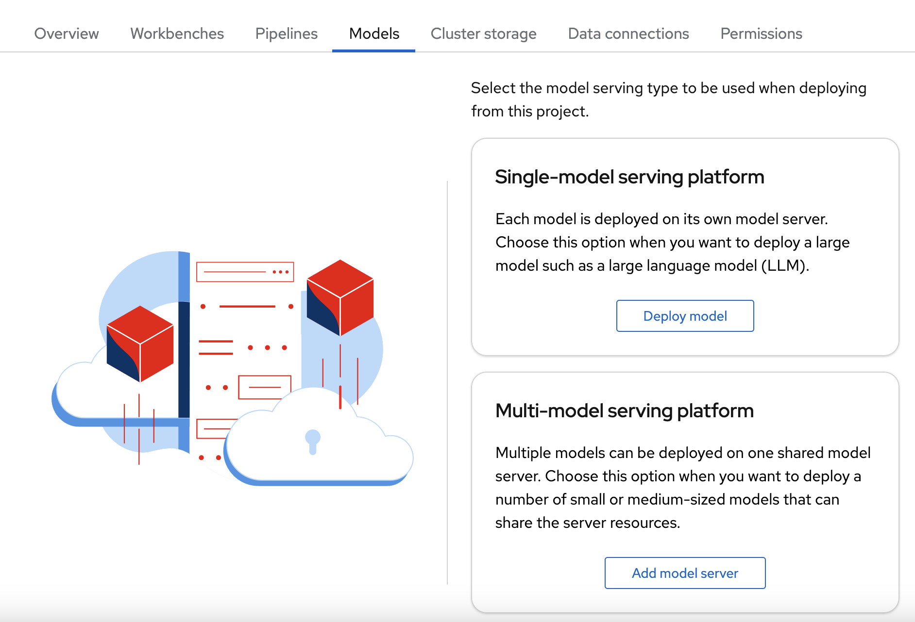
- In the Single-model serving platform tile, click Deploy model.
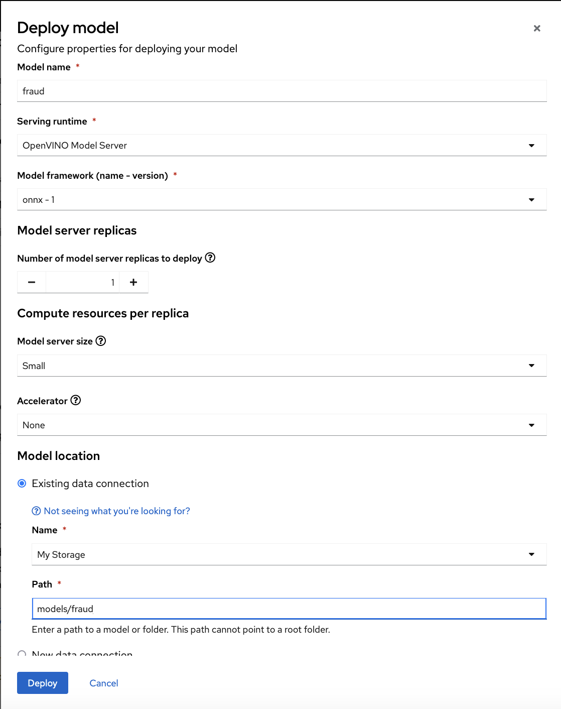
In the form, provide the following values:
-
For Model Name, type
fraud. -
For Serving runtime, select
OpenVINO Model Server. -
For Model framework, select
onnx-1. -
For Existing data connection, select
My Storage. -
Type the path that leads to the version folder that contains your model file:
models/fraud Leave the other fields with the default settings.
-
For Model Name, type
- Click Deploy.
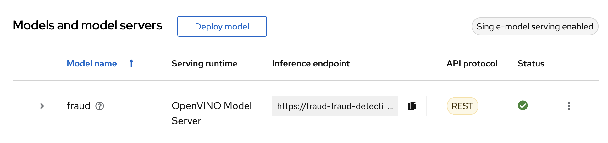
Verification
Wait for the model to deploy and for the Status to show a green checkmark.
Next step
4.2.2. Deploying a model on a multi-model server
OpenShift AI multi-model servers can host several models at once. You create a new model server and deploy your model to it.
Prerequiste
-
A user with
adminprivileges has enabled the multi-model serving platform on your OpenShift cluster.
Procedure
In the OpenShift AI dashboard, navigate to the project details page and click the Models tab.
- In the Multi-model serving platform tile, click Add model server.
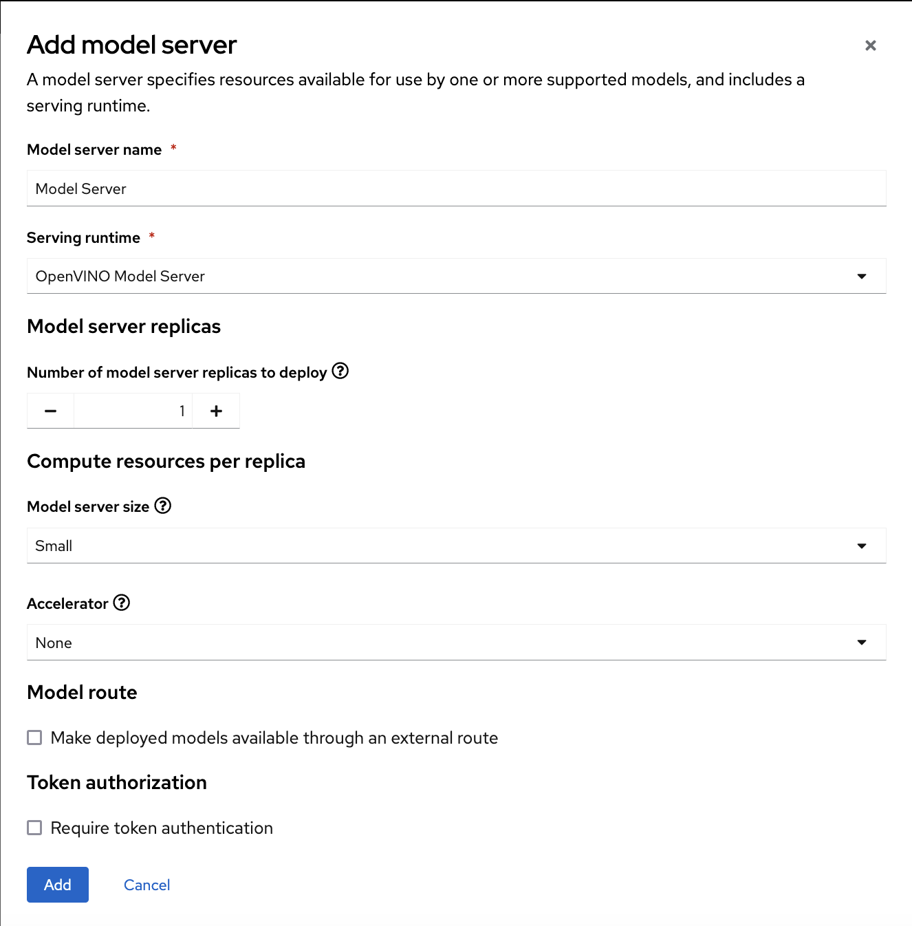
In the form, provide the following values:
-
For Model server name, type a name, for example
Model Server. -
For Serving runtime, select
OpenVINO Model Server. Leave the other fields with the default settings.
-
For Model server name, type a name, for example
- Click Add.
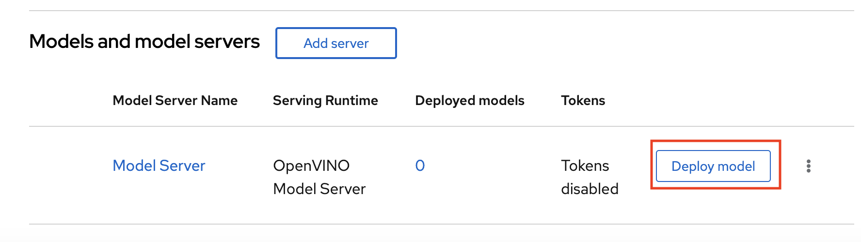
In the Models and model servers list, next to the new model server, click Deploy model.
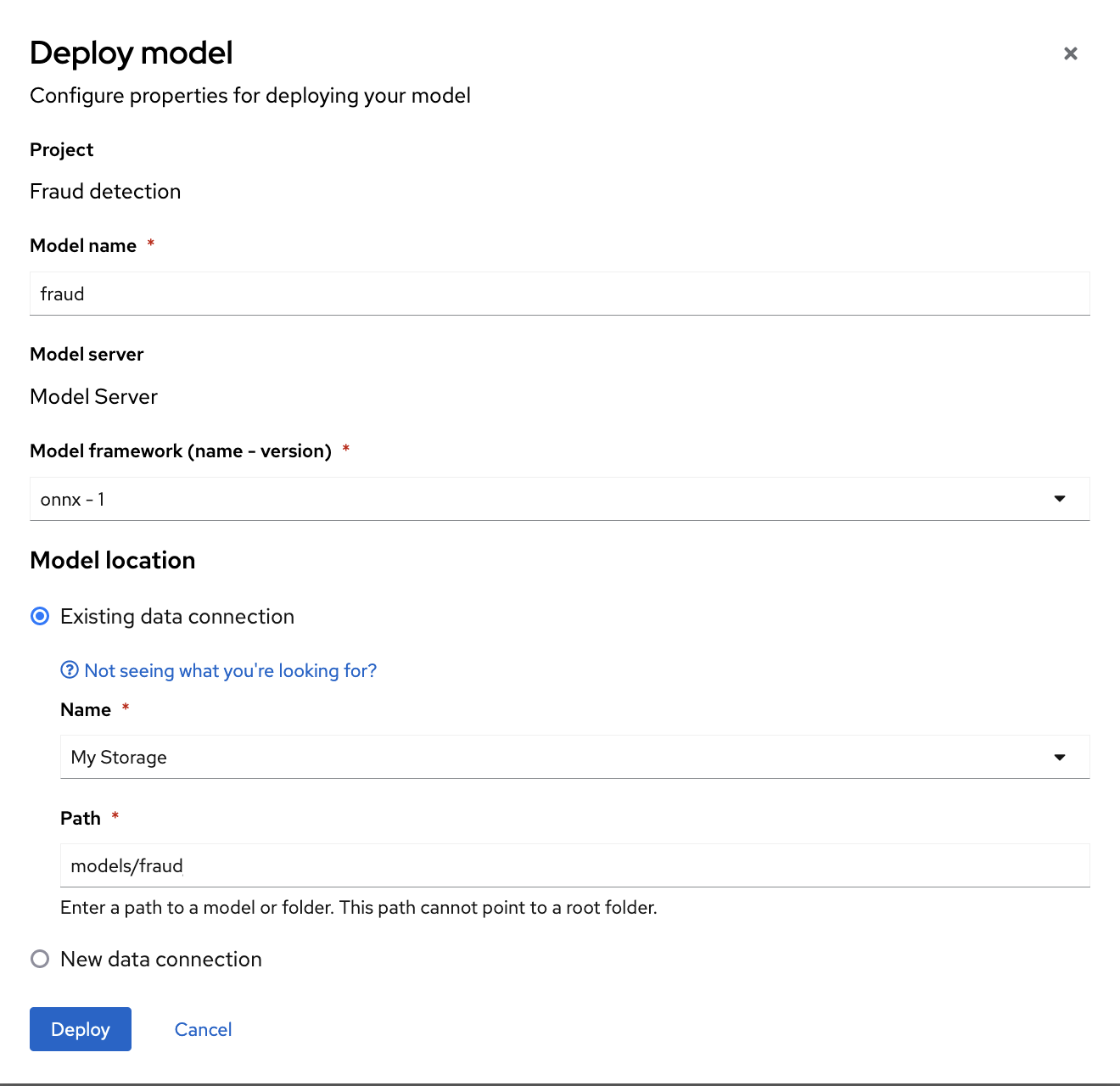
In the form, provide the following values:
-
For Model Name, type
fraud. -
For Model framework, select
onnx-1. -
For Existing data connection, select
My Storage. -
Type the path that leads to the version folder that contains your model file:
models/fraud Leave the other fields with the default settings.
-
For Model Name, type
- Click Deploy.
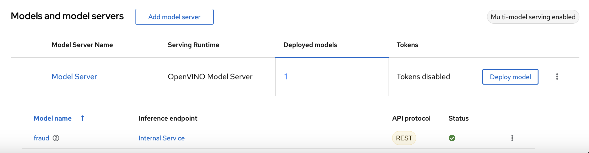
Verification
Wait for the model to deploy and for the Status to show a green checkmark.
Next step
4.3. Testing the model API
Now that you’ve deployed the model, you can test its API endpoints.
Procedure
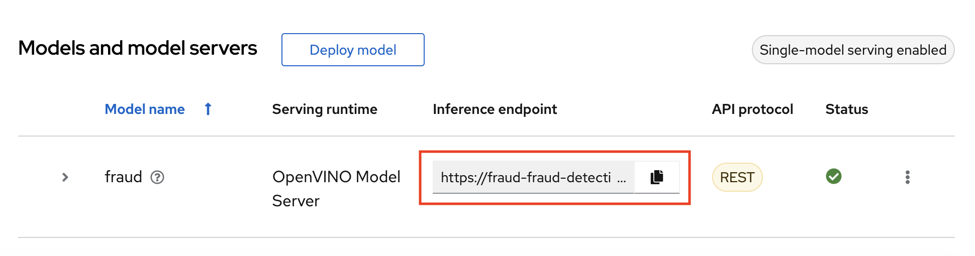
- In the OpenShift AI dashboard, navigate to the project details page and click the Models tab.
Take note of the model’s Inference endpoint. You need this information when you test the model API.
Return to the Jupyter environment and try out your new endpoint.
If you deployed your model with multi-model serving, follow the directions in
3_rest_requests_multi_model.ipynbto try a REST API call and4_grpc_requests_multi_model.ipynbto try a gRPC API call.If you deployed your model with single-model serving, follow the directions in
5_rest_requests_single_model.ipynbto try a REST API call.
Chapter 5. Implementing pipelines
5.1. Automating workflows with data science pipelines
In previous sections of this tutorial, you used a notebook to train and save your model. Optionally, you can automate these tasks by using Red Hat OpenShift AI pipelines. Pipelines offer a way to automate the execution of multiple notebooks and Python code. By using pipelines, you can execute long training jobs or retrain your models on a schedule without having to manually run them in a notebook.
In this section, you create a simple pipeline by using the GUI pipeline editor. The pipeline uses the notebook that you used in previous sections to train a model and then save it to S3 storage.
Your completed pipeline should look like the one in the 6 Train Save.pipeline file.
Note: You can run and use 6 Train Save.pipeline. To explore the pipeline editor, complete the steps in the following procedure to create your own pipeline.
5.1.1. Create a pipeline
Open your workbench’s JupyterLab environment. If the launcher is not visible, click + to open it.
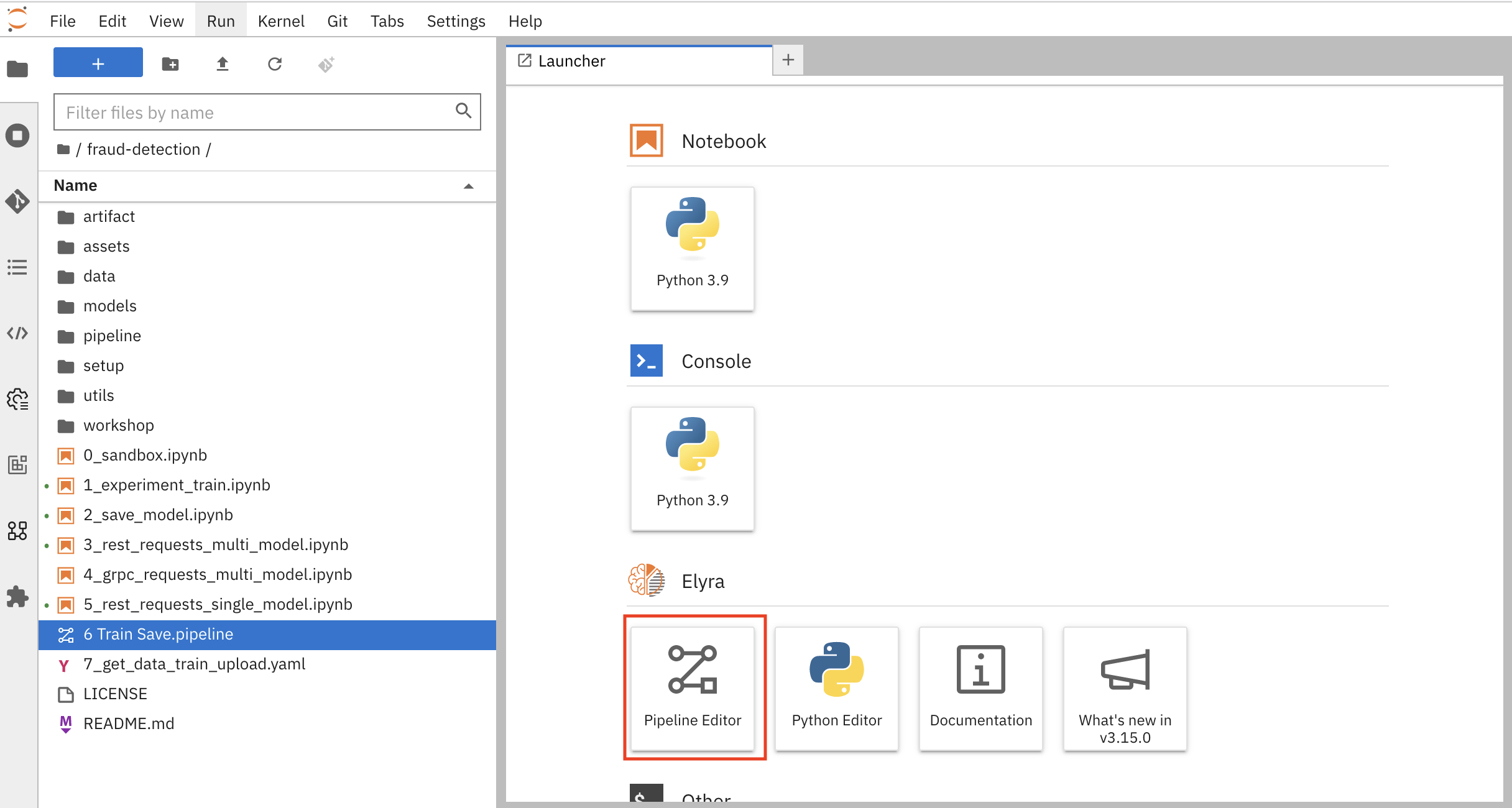
Click Pipeline Editor.
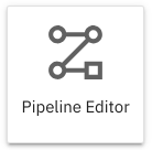
You’ve created a blank pipeline!
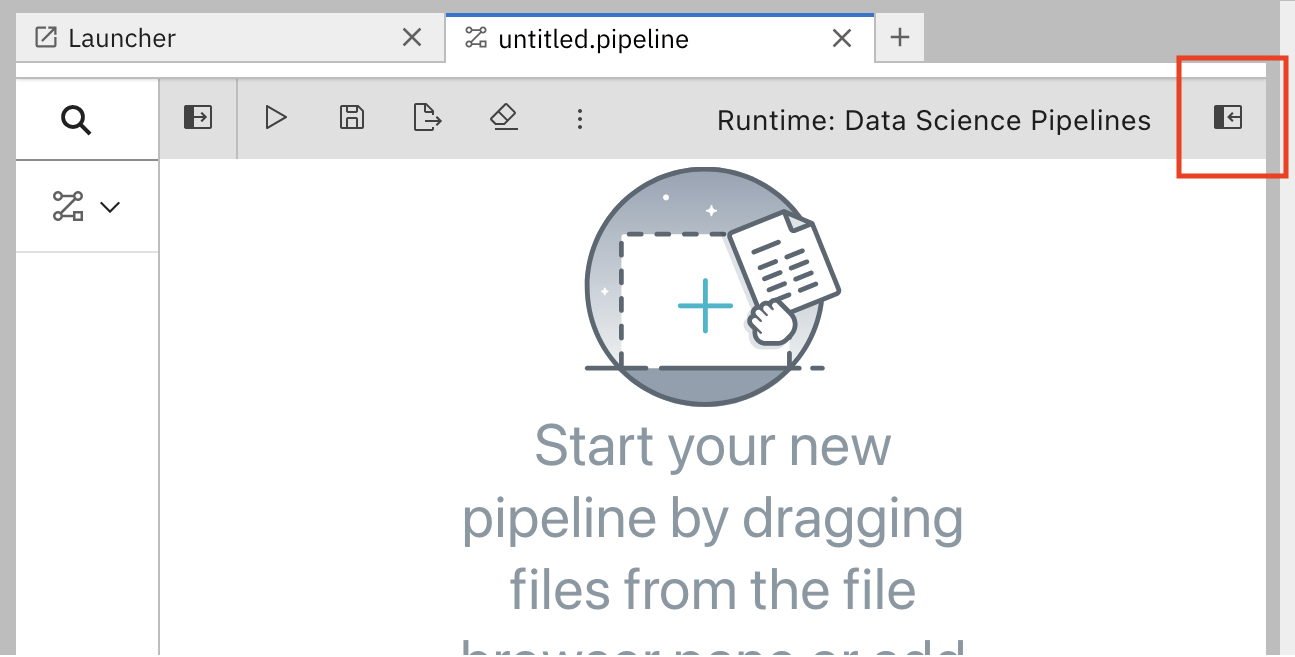
Set the default runtime image for when you run your notebook or Python code.
In the pipeline editor, click Open Panel.
Select the Pipeline Properties tab.
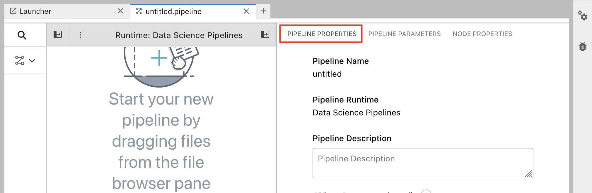
In the Pipeline Properties panel, scroll down to Generic Node Defaults and Runtime Image. Set the value to
Tensorflow with Cuda and Python 3.9 (UBI 9).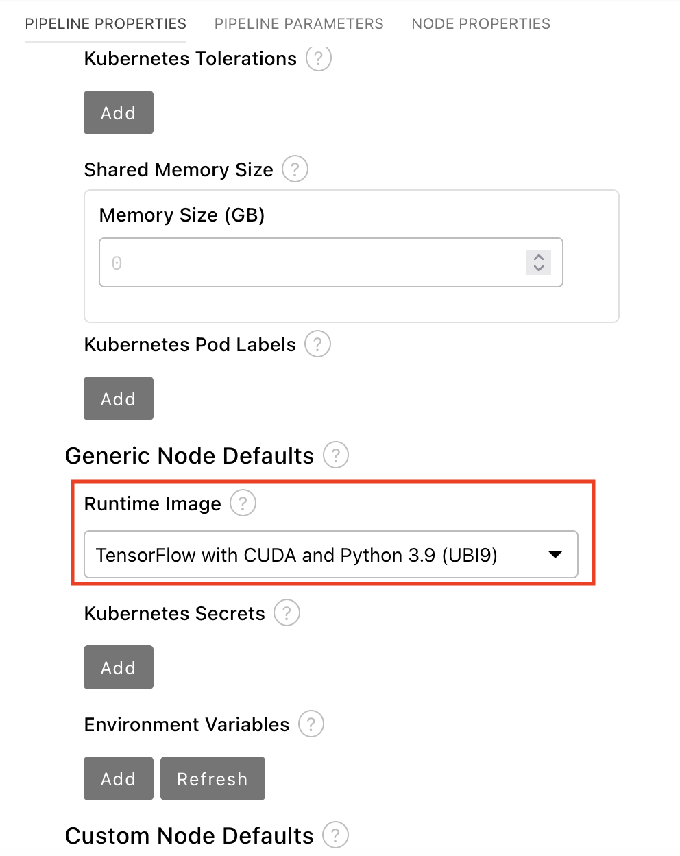
- Save the pipeline.
5.1.2. Add nodes to your pipeline
Add some steps, or nodes in your pipeline. Your two nodes will use the 1_experiment_train.ipynb and 2_save_model.ipynb notebooks.
From the file-browser panel, drag the
1_experiment_train.ipynband2_save_model.ipynbnotebooks onto the pipeline canvas.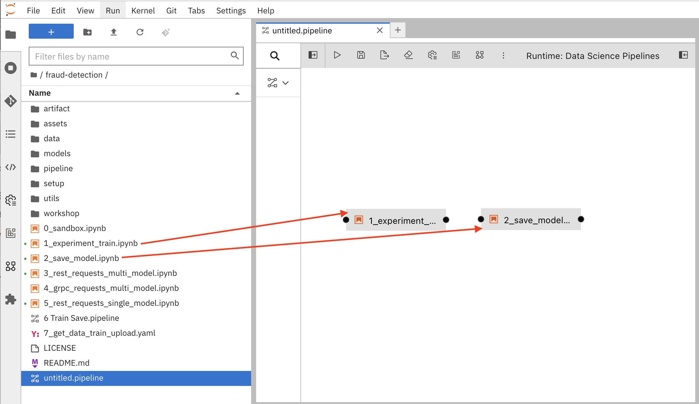
Click the output port of
1_experiment_train.ipynband drag a connecting line to the input port of2_save_model.ipynb.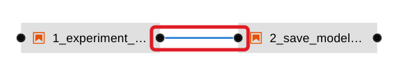
- Save the pipeline.
5.1.3. Specify the training file as a dependency
Set node properties to specify the training file as a dependency.
Note: If you don’t set this file dependency, the file is not included in the node when it runs and the training job fails.
Click the
1_experiment_train.ipynbnode.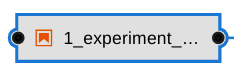
- In the Properties panel, click the Node Properties tab.
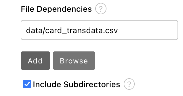
Scroll down to the File Dependencies section and then click Add.
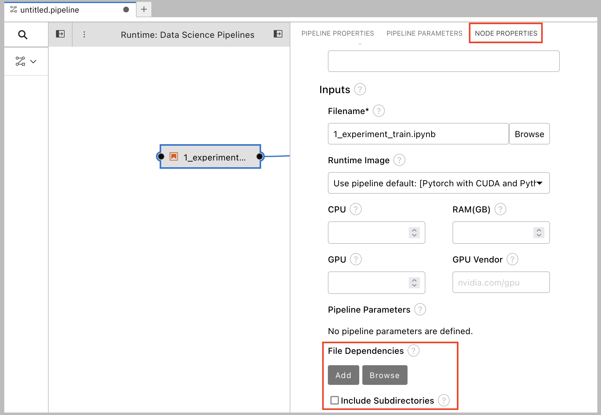
-
Set the value to
data/card_transdata.csvwhich contains the data to train your model. Select the Include Subdirectories option and then click Add.
- Save the pipeline.
5.1.4. Create and store the ONNX-formatted output file
In node 1, the notebook creates the models/fraud/1/model.onnx file. In node 2, the notebook uploads that file to the S3 storage bucket. You must set models/fraud/1/model.onnx file as the output file for both nodes.
- Select node 1 and then select the Node Properties tab.
- Scroll down to the Output Files section, and then click Add.
Set the value to
models/fraud/1/model.onnxand then click Add.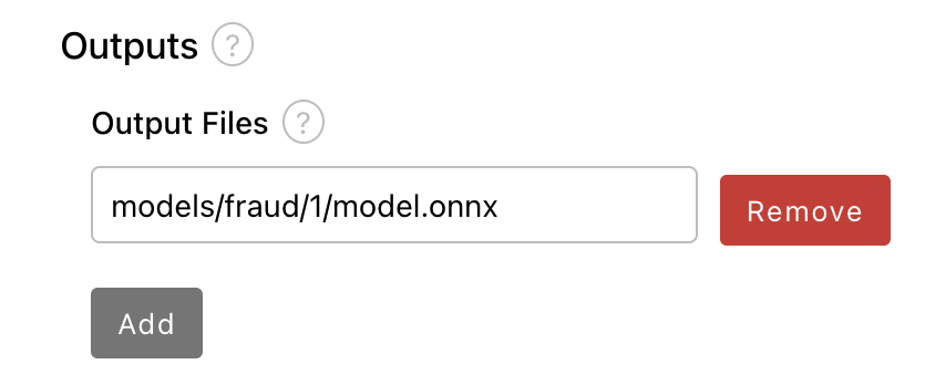
- Repeat steps 1-3 for node 2.
- Save the pipeline.
5.1.5. Configure the data connection to the S3 storage bucket
In node 2, the notebook uploads the model to the S3 storage bucket.
You must set the S3 storage bucket keys by using the secret created by the My Storage data connection that you set up in the Storing data with data connections section of this tutorial.
You can use this secret in your pipeline nodes without having to save the information in your pipeline code. This is important, for example, if you want to save your pipelines - without any secret keys - to source control.
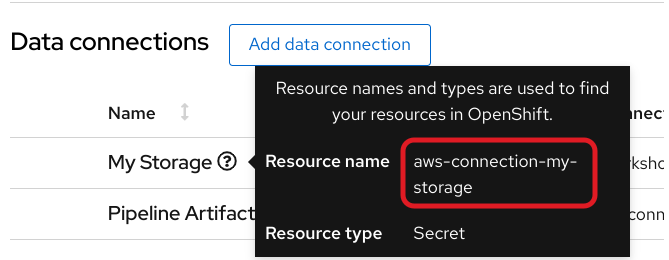
The secret is named aws-connection-my-storage.
If you named your data connection something other than My Storage, you can obtain the secret name in the OpenShift AI dashboard by hovering over the resource information icon ? in the Data Connections tab.
The aws-connection-my-storage secret includes the following fields:
-
AWS_ACCESS_KEY_ID -
AWS_DEFAULT_REGION -
AWS_S3_BUCKET -
AWS_S3_ENDPOINT -
AWS_SECRET_ACCESS_KEY
You must set the secret name and key for each of these fields.
Procedure
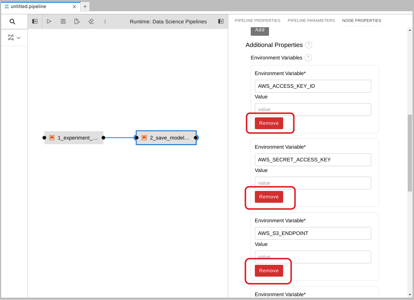
Remove any pre-filled environment variables.
Select node 2, and then select the Node Properties tab.
Under Additional Properties, note that some environment variables have been pre-filled. The pipeline editor inferred that you need them from the notebook code.
Since you don’t want to save the value in your pipelines, remove all of these environment variables.
Click Remove for each of the pre-filled environment variables.
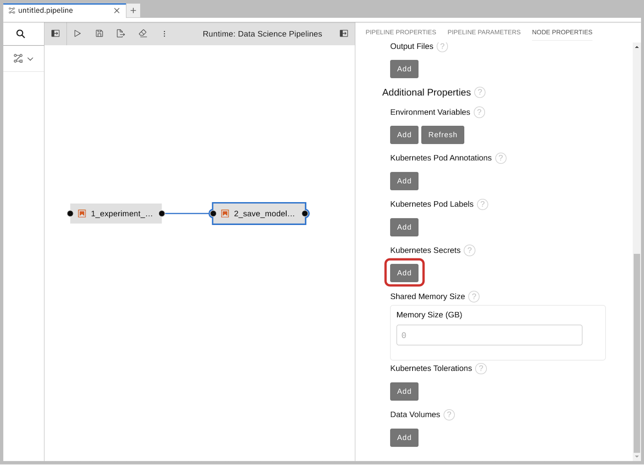
Add the S3 bucket and keys by using the Kubernetes secret.
Under Kubernetes Secrets, click Add.
Enter the following values and then click Add.
-
Environment Variable:
AWS_ACCESS_KEY_ID -
Secret Name:
aws-connection-my-storage Secret Key:
AWS_ACCESS_KEY_ID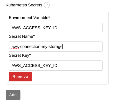
-
Environment Variable:
Repeat Steps 2a and 2b for each set of these Kubernetes secrets:
Environment Variable:
AWS_SECRET_ACCESS_KEY-
Secret Name:
aws-connection-my-storage -
Secret Key:
AWS_SECRET_ACCESS_KEY
-
Secret Name:
Environment Variable:
AWS_S3_ENDPOINT-
Secret Name:
aws-connection-my-storage -
Secret Key:
AWS_S3_ENDPOINT
-
Secret Name:
Environment Variable:
AWS_DEFAULT_REGION-
Secret Name:
aws-connection-my-storage -
Secret Key:
AWS_DEFAULT_REGION
-
Secret Name:
Environment Variable:
AWS_S3_BUCKET-
Secret Name:
aws-connection-my-storage -
Secret Key:
AWS_S3_BUCKET
-
Secret Name:
-
Save and Rename the
.pipelinefile.
5.1.6. Run the Pipeline
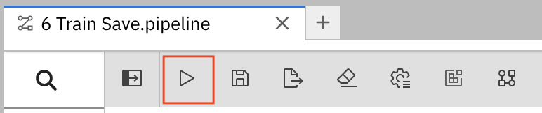
Upload the pipeline on your cluster and run it. You can do so directly from the pipeline editor. You can use your own newly created pipeline for this or 6 Train Save.pipeline.
Procedure
Click the play button in the toolbar of the pipeline editor.
- Enter a name for your pipeline.
-
Verify the Runtime Configuration: is set to
Data Science Pipeline. Click OK.
NoteIf
Data Science Pipelineis not available as a runtime configuration, you may have created your notebook before the pipeline server was available. You can restart your notebook after the pipeline server has been created in your data science project.Return to your data science project and expand the newly created pipeline.
Click View runs and then view the pipeline run in progress.
The result should be a models/fraud/1/model.onnx file in your S3 bucket which you can serve, just like you did manually in the Preparing a model for deployment section.
Next step
5.2. Running a data science pipeline generated from Python code
In the previous section, you created a simple pipeline by using the GUI pipeline editor. It’s often desirable to create pipelines by using code that can be version-controlled and shared with others. The kfp SDK provides a Python API for creating pipelines. The SDK is available as a Python package that you can install by using the pip install kfp command. With this package, you can use Python code to create a pipeline and then compile it to YAML format. Then you can import the YAML code into OpenShift AI.
This tutorial does not delve into the details of how to use the SDK. Instead, it provides the files for you to view and upload.
Optionally, view the provided Python code in your Jupyter environment by navigating to the
fraud-detection-notebooksproject’spipelinedirectory. It contains the following files:-
7_get_data_train_upload.pyis the main pipeline code. -
get_data.py,train_model.py, andupload.pyare the three components of the pipeline. build.shis a script that builds the pipeline and creates the YAML file.For your convenience, the output of the
build.shscript is provided in the7_get_data_train_upload.yamlfile. The7_get_data_train_upload.yamloutput file is located in the top-levelfraud-detectiondirectory.
-
-
Right-click the
7_get_data_train_upload.yamlfile and then click Download. Upload the
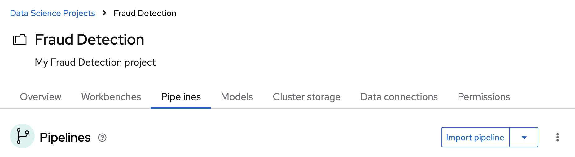
7_get_data_train_upload.yamlfile to OpenShift AI.In the OpenShift AI dashboard, navigate to your data science project page. Click the Pipelines tab and then click Import pipeline.
- Enter values for Pipeline name and Pipeline description.
Click Upload and then select
7_get_data_train_upload.yamlfrom your local files to upload the pipeline.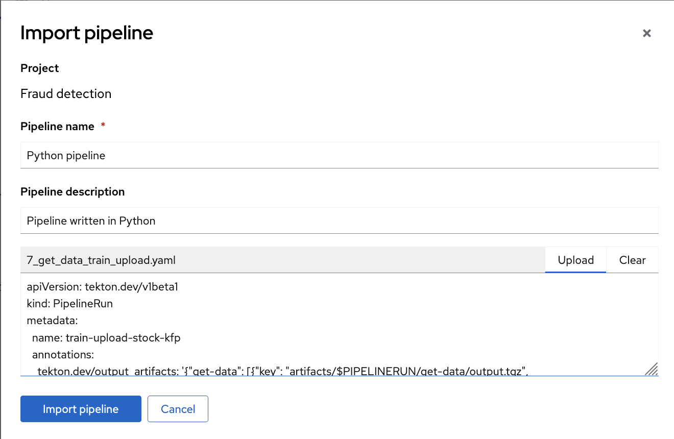
Click Import pipeline to import and save the pipeline.
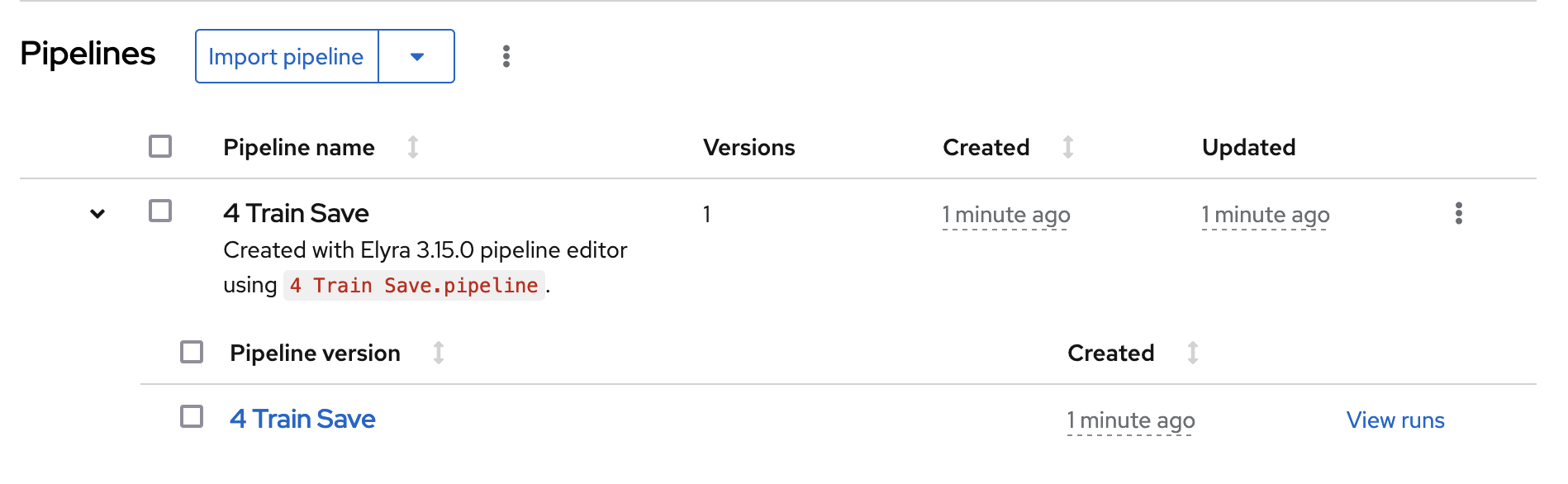
The pipeline shows in the list of pipelines.
Expand the pipeline item, click the action menu (⋮), and then select View runs.
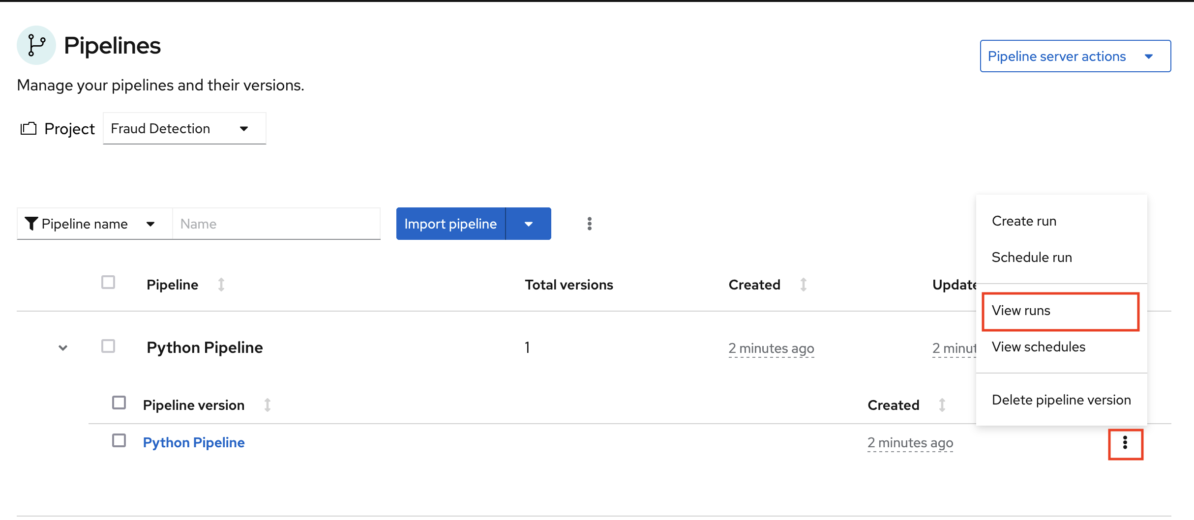
- Click Create run.
On the Create run page, provide the following values:
-
For Name, type any name, for example
Run 1. For Pipeline, select the pipeline that you uploaded.
You can leave the other fields with their default values.
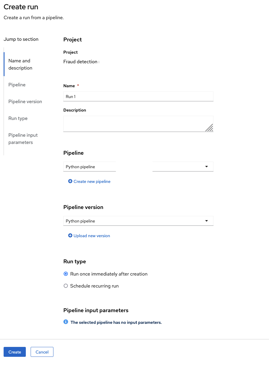
-
For Name, type any name, for example
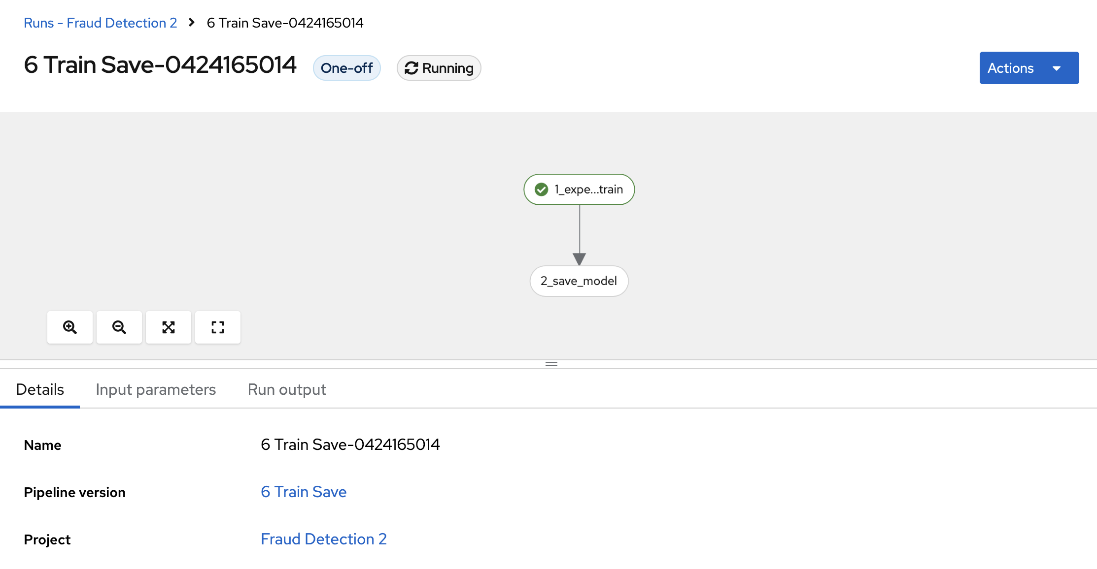
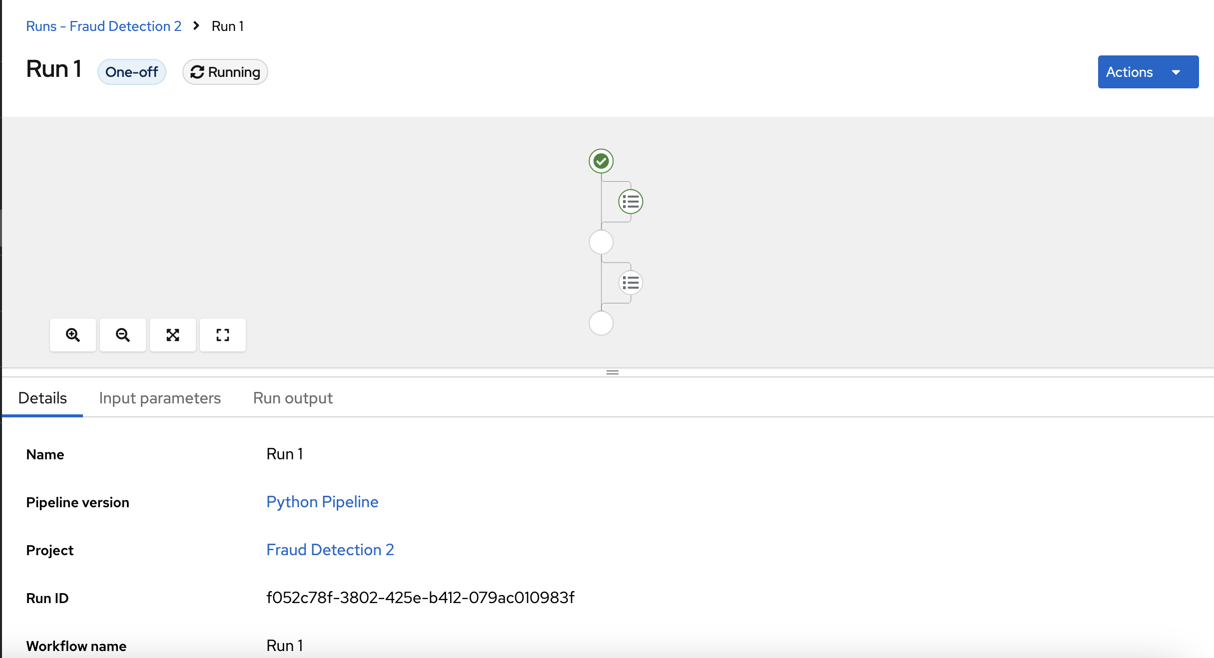
Click Create to create the run.
A new run starts immediately. The Details page shows a pipeline created in Python that is running in OpenShift AI.
Chapter 6. Conclusion
Congratulations!
In this tutorial, you learned how to incorporate data science and artificial intelligence (AI) and machine learning (ML) into an OpenShift development workflow.
You used an example fraud detection model and completed the following tasks:
- Explored a pre-trained fraud detection model by using a Jupyter notebook.
- Deployed the model by using OpenShift AI model serving.
- Refined and trained the model by using automated pipelines.