
Developing solvers with Red Hat Business Optimizer in Red Hat Process Automation Manager
Abstract
Preface
As a developer of business decisions and processes , you can use Red Hat Business Optimizer to develop solvers that determine the optimal solution to planning problems. Red Hat Business Optimizer is a built-in component of Red Hat Process Automation Manager. You can use solvers as part of your services in Red Hat Process Automation Manager to optimize limited resources with specific constraints.
Making open source more inclusive
Red Hat is committed to replacing problematic language in our code, documentation, and web properties. We are beginning with these four terms: master, slave, blacklist, and whitelist. Because of the enormity of this endeavor, these changes will be implemented gradually over several upcoming releases. For more details, see our CTO Chris Wright’s message.
Part I. Getting started with Red Hat Business Optimizer
As a business rules developer, you can use the Red Hat Business Optimizer to find the optimal solution to planning problems based on a set of limited resources and under specific constraints.
Use this document to start developing solvers with Red Hat Business Optimizer.
Chapter 1. Introduction to Red Hat Business Optimizer
Red Hat Business Optimizer is a lightweight, embeddable planning engine that optimizes planning problems. It helps normal Java programmers solve planning problems efficiently, and it combines optimization heuristics and metaheuristics with very efficient score calculations.
For example, Red Hat Business Optimizer helps solve various use cases:
- Employee/Patient Rosters: It helps create timetables for nurses and keeps track of patient bed management.
- Educational Timetables: It helps schedule lessons, courses, exams, and conference presentations.
- Shop Schedules: It tracks car assembly lines, machine queue planning, and workforce task planning.
- Cutting Stock: It minimizes waste by reducing the consumption of resources such as paper and steel.
Every organization faces planning problems; that is, they provide products and services with a limited set of constrained resources (employees, assets, time, and money).
Red Hat Business Optimizer is open source software under the Apache Software License 2.0. It is 100% pure Java and runs on most Java virtual machines.
1.1. Planning problems
A planning problem has an optimal goal, based on limited resources and under specific constraints. Optimal goals can be any number of things, such as:
- Maximized profits - the optimal goal results in the highest possible profit.
- Minimized ecological footprint - the optimal goal has the least amount of environmental impact.
- Maximized satisfaction for employees or customers - the optimal goal prioritizes the needs of employees or customers.
The ability to achieve these goals relies on the number of resources available. For example, the following resources might be limited:
- The number of people
- Amount of time
- Budget
- Physical assets, for example, machinery, vehicles, computers, buildings, and so on
You must also take into account the specific constraints related to these resources, such as the number of hours a person works, their ability to use certain machines, or compatibility between pieces of equipment.
Red Hat Business Optimizer helps Java programmers solve constraint satisfaction problems efficiently. It combines optimization heuristics and metaheuristics with efficient score calculation.
1.2. NP-completeness in planning problems
The provided use cases are probably NP-complete or NP-hard, which means the following statements apply:
- It is easy to verify a given solution to a problem in reasonable time.
- There is no simple way to find the optimal solution of a problem in reasonable time.
The implication is that solving your problem is probably harder than you anticipated, because the two common techniques do not suffice:
- A brute force algorithm (even a more advanced variant) takes too long.
- A quick algorithm, for example in the bin packing problem, putting in the largest items first returns a solution that is far from optimal.
By using advanced optimization algorithms, Business Optimizer finds a good solution in reasonable time for such planning problems.
1.3. Solutions to planning problems
A planning problem has a number of solutions.
Several categories of solutions are:
- Possible solution
- A possible solution is any solution, whether or not it breaks any number of constraints. Planning problems often have an incredibly large number of possible solutions. Many of those solutions are not useful.
- Feasible solution
- A feasible solution is a solution that does not break any (negative) hard constraints. The number of feasible solutions are relative to the number of possible solutions. Sometimes there are no feasible solutions. Every feasible solution is a possible solution.
- Optimal solution
- An optimal solution is a solution with the highest score. Planning problems usually have a few optimal solutions. They always have at least one optimal solution, even in the case that there are no feasible solutions and the optimal solution is not feasible.
- Best solution found
- The best solution is the solution with the highest score found by an implementation in a given amount of time. The best solution found is likely to be feasible and, given enough time, it’s an optimal solution.
Counterintuitively, the number of possible solutions is huge (if calculated correctly), even with a small data set.
In the examples provided in the planner-engine distribution folder, most instances have a large number of possible solutions. As there is no guaranteed way to find the optimal solution, any implementation is forced to evaluate at least a subset of all those possible solutions.
Business Optimizer supports several optimization algorithms to efficiently wade through that incredibly large number of possible solutions.
Depending on the use case, some optimization algorithms perform better than others, but it is impossible to know in advance. Using Business Optimizer, you can switch the optimization algorithm by changing the solver configuration in a few lines of XML or code.
1.4. Constraints on planning problems
Usually, a planning problem has minimum two levels of constraints:
A (negative) hard constraint must not be broken.
For example, one teacher can not teach two different lessons at the same time.
A (negative) soft constraint should not be broken if it can be avoided.
For example, Teacher A does not like to teach on Friday afternoons.
Some problems also have positive constraints:
A positive soft constraint (or reward) should be fulfilled if possible.
For example, Teacher B likes to teach on Monday mornings.
Some basic problems only have hard constraints. Some problems have three or more levels of constraints, for example, hard, medium, and soft constraints.
These constraints define the score calculation (otherwise known as the fitness function) of a planning problem. Each solution of a planning problem is graded with a score. With Business Optimizer, score constraints are written in an object oriented language such as Java, or in Drools rules.
This type of code is flexible and scalable.
Chapter 2. Getting started with solvers in Business Central: An employee rostering example
You can build and deploy the employee-rostering sample project in Business Central. The project demonstrates how to create each of the Business Central assets required to solve the shift rostering planning problem and use Red Hat Business Optimizer to find the best possible solution.
You can deploy the preconfigured employee-rostering project in Business Central. Alternatively, you can create the project yourself using Business Central.
The employee-rostering sample project in Business Central does not include a data set. You must supply a data set in XML format using a REST API call.
2.1. Deploying the employee rostering sample project in Business Central
Business Central includes a number of sample projects that you can use to get familiar with the product and its features. The employee rostering sample project is designed and created to demonstrate the shift rostering use case for Red Hat Business Optimizer. Use the following procedure to deploy and run the employee rostering sample in Business Central.
Prerequisites
- Red Hat Process Automation Manager has been downloaded and installed. For installation options, see Planning a Red Hat Process Automation Manager installation.
-
You have started Red Hat Process Automation Manager, as described in the installation documentation, and you are logged in to Business Central as a user with
adminpermissions.
Procedure
- In Business Central, click Menu → Design → Projects.
-
In the preconfigured
MySpacespace, click Try Samples. - Select employee-rostering from the list of sample projects and click Ok in the upper-right corner to import the project.
- After the asset list has complied, click Build & Deploy to deploy the employee rostering example.
The rest of this document explains each of the project assets and their configuration.
2.2. Re-creating the employee rostering sample project
The employee rostering sample project is a preconfigured project available in Business Central. You can learn about how to deploy this project in Section 2.1, “Deploying the employee rostering sample project in Business Central”.
You can create the employee rostering example "from scratch". You can use the workflow in this example to create a similar project of your own in Business Central.
2.2.1. Setting up the employee rostering project
To start developing a solver in Business Central, you must set up the project.
Prerequisites
- Red Hat Process Automation Manager has been downloaded and installed.
-
You have deployed Business Central and logged in with a user that has the
adminrole.
Procedure
- Create a new project in Business Central by clicking Menu → Design → Projects → Add Project.
In the Add Project window, fill out the following fields:
-
Name:
employee-rostering - Description(optional): Employee rostering problem optimization using Business Optimizer. Assigns employees to shifts based on their skill.
Optionally, click Configure Advanced Options to populate the
Group ID,Artifact ID, andVersioninformation.-
Group ID:
employeerostering -
Artifact ID:
employeerostering -
Version:
1.0.0-SNAPSHOT
-
Name:
- Click Add to add the project to the Business Central project repository.
2.2.2. Problem facts and planning entities
Each of the domain classes in the employee rostering planning problem is categorized as one of the following:
- An unrelated class: not used by any of the score constraints. From a planning standpoint, this data is obsolete.
-
A problem fact class: used by the score constraints, but does not change during planning (as long as the problem stays the same), for example,
ShiftandEmployee. All the properties of a problem fact class are problem properties. A planning entity class: used by the score constraints and changes during planning, for example,
ShiftAssignment. The properties that change during planning are planning variables. The other properties are problem properties.Ask yourself the following questions:
- What class changes during planning?
Which class has variables that I want the
Solverto change?That class is a planning entity.
A planning entity class needs to be annotated with the
@PlanningEntityannotation, or defined in Business Central using the Red Hat Business Optimizer dock in the domain designer.Each planning entity class has one or more planning variables, and must also have one or more defining properties.
Most use cases have only one planning entity class, and only one planning variable per planning entity class.
2.2.3. Creating the data model for the employee rostering project
Use this section to create the data objects required to run the employee rostering sample project in Business Central.
Prerequisites
- You have completed the project setup described in Section 2.2.1, “Setting up the employee rostering project”.
Procedure
- With your new project, either click Data Object in the project perspective, or click Add Asset → Data Object to create a new data object.
Name the first data object
Timeslot, and selectemployeerostering.employeerosteringas the Package.Click Ok.
-
In the Data Objects perspective, click +add field to add fields to the
Timeslotdata object. -
In the id field, type
endTime. -
Click the drop-down menu next to Type and select
LocalDateTime. - Click Create and continue to add another field.
-
Add another field with the id
startTimeand TypeLocalDateTime. - Click Create.
-
Click Save in the upper-right corner to save the
Timeslotdata object. - Click the x in the upper-right corner to close the Data Objects perspective and return to the Assets menu.
Using the previous steps, create the following data objects and their attributes:
Table 2.1. Skill
id Type nameStringTable 2.2. Employee
id Type nameStringskillsemployeerostering.employeerostering.Skill[List]Table 2.3. Shift
id Type requiredSkillemployeerostering.employeerostering.Skilltimeslotemployeerostering.employeerostering.TimeslotTable 2.4. DayOffRequest
id Type dateLocalDateemployeeemployeerostering.employeerostering.EmployeeTable 2.5. ShiftAssignment
id Type employeeemployeerostering.employeerostering.Employeeshiftemployeerostering.employeerostering.Shift
For more examples of creating data objects, see Getting started with decision services.
2.2.3.1. Creating the employee roster planning entity
In order to solve the employee rostering planning problem, you must create a planning entity and a solver. The planning entity is defined in the domain designer using the attributes available in the Red Hat Business Optimizer dock.
Use the following procedure to define the ShiftAssignment data object as the planning entity for the employee rostering example.
Prerequisites
- You have created the relevant data objects and planning entity required to run the employee rostering example by completing the procedures in Section 2.2.3, “Creating the data model for the employee rostering project”.
Procedure
-
From the project Assets menu, open the
ShiftAssignmentdata object. -
In the Data Objects perspective, open the Red Hat Business Optimizer dock by clicking the
 on the right.
- Select Planning Entity.
-
Select
employeefrom the list of fields under theShiftAssignmentdata object. In the Red Hat Business Optimizer dock, select Planning Variable.
In the Value Range Id input field, type
employeeRange. This adds the@ValueRangeProviderannotation to the planning entity, which you can view by clicking theSourcetab in the designer.The value range of a planning variable is defined with the
@ValueRangeProviderannotation. A@ValueRangeProviderannotation always has a propertyid, which is referenced by the@PlanningVariablepropertyvalueRangeProviderRefs.- Close the dock and click Save to save the data object.
2.2.3.2. Creating the employee roster planning solution
The employee roster problem relies on a defined planning solution. The planning solution is defined in the domain designer using the attributes available in the Red Hat Business Optimizer dock.
Prerequisites
- You have created the relevant data objects and planning entity required to run the employee rostering example by completing the procedures in Section 2.2.3, “Creating the data model for the employee rostering project” and Section 2.2.3.1, “Creating the employee roster planning entity”.
Procedure
-
Create a new data object with the identifier
EmployeeRoster. Create the following fields:
Table 2.6. EmployeeRoster
id Type dayOffRequestListemployeerostering.employeerostering.DayOffRequest[List]shiftAssignmentListemployeerostering.employeerostering.ShiftAssignment[List]shiftListemployeerostering.employeerostering.Shift[List]skillListemployeerostering.employeerostering.Skill[List]timeslotListemployeerostering.employeerostering.Timeslot[List]-
In the Data Objects perspective, open the Red Hat Business Optimizer dock by clicking the
on the right.
- Select Planning Solution.
-
Leave the default
Hard soft scoreas the Solution Score Type. This automatically generates ascorefield in theEmployeeRosterdata object with the solution score as the type. Add a new field with the following attributes:
id Type employeeListemployeerostering.employeerostering.Employee[List]With the
employeeListfield selected, open the Red Hat Business Optimizer dock and select the Planning Value Range Provider box.In the id field, type
employeeRange. Close the dock.- Click Save in the upper-right corner to save the asset.
2.2.4. Employee rostering constraints
Employee rostering is a planning problem. All planning problems include constraints that must be satisfied in order to find an optimal solution.
The employee rostering sample project in Business Central includes the following hard and soft constraints:
- Hard constraint
- Employees are only assigned one shift per day.
- All shifts that require a particular employee skill are assigned an employee with that particular skill.
- Soft constraints
- All employees are assigned a shift.
- If an employee requests a day off, their shift is reassigned to another employee.
Hard and soft constraints are defined in Business Central using either the free-form DRL designer, or using guided rules.
2.2.4.1. DRL (Drools Rule Language) rules
DRL (Drools Rule Language) rules are business rules that you define directly in .drl text files. These DRL files are the source in which all other rule assets in Business Central are ultimately rendered. You can create and manage DRL files within the Business Central interface, or create them externally as part of a Maven or Java project using Red Hat CodeReady Studio or another integrated development environment (IDE). A DRL file can contain one or more rules that define at a minimum the rule conditions (when) and actions (then). The DRL designer in Business Central provides syntax highlighting for Java, DRL, and XML.
DRL files consist of the following components:
Components in a DRL file
package

import

function  // Optional

query  // Optional

declare   // Optional

global   // Optional

rule "rule name"
    // Attributes
    when
        // Conditions
    then
        // Actions
end

rule "rule2 name"

...
The following example DRL rule determines the age limit in a loan application decision service:
Example rule for loan application age limit
rule "Underage"
  salience 15
  agenda-group "applicationGroup"
  when
    $application : LoanApplication()
    Applicant( age < 21 )
  then
    $application.setApproved( false );
    $application.setExplanation( "Underage" );
end
A DRL file can contain single or multiple rules, queries, and functions, and can define resource declarations such as imports, globals, and attributes that are assigned and used by your rules and queries. The DRL package must be listed at the top of a DRL file and the rules are typically listed last. All other DRL components can follow any order.
Each rule must have a unique name within the rule package. If you use the same rule name more than once in any DRL file in the package, the rules fail to compile. Always enclose rule names with double quotation marks (rule "rule name") to prevent possible compilation errors, especially if you use spaces in rule names.
All data objects related to a DRL rule must be in the same project package as the DRL file in Business Central. Assets in the same package are imported by default. Existing assets in other packages can be imported with the DRL rule.
2.2.4.2. Defining constraints for employee rostering using the DRL designer
You can create constraint definitions for the employee rostering example using the free-form DRL designer in Business Central.
Use this procedure to create a hard constraint where no employee is assigned a shift that begins less than 10 hours after their previous shift ended.
Procedure
- In Business Central, go to Menu → Design → Projects and click the project name.
- Click Add Asset → DRL file.
-
In the DRL file name field, type
ComplexScoreRules. -
Select the
employeerostering.employeerosteringpackage. - Click +Ok to create the DRL file.
In the Model tab of the DRL designer, define the
Employee10HourShiftSpacerule as a DRL file:package employeerostering.employeerostering; rule "Employee10HourShiftSpace" when $shiftAssignment : ShiftAssignment( $employee : employee != null, $shiftEndDateTime : shift.timeslot.endTime) ShiftAssignment( this != $shiftAssignment, $employee == employee, $shiftEndDateTime <= shift.timeslot.endTime, $shiftEndDateTime.until(shift.timeslot.startTime, java.time.temporal.ChronoUnit.HOURS) <10) then scoreHolder.addHardConstraintMatch(kcontext, -1); end- Click Save to save the DRL file.
For more information about creating DRL files, see Designing a decision service using DRL rules.
2.2.5. Creating rules for employee rostering using guided rules
You can create rules that define hard and soft constraints for employee rostering using the guided rules designer in Business Central.
2.2.5.1. Guided rules
Guided rules are business rules that you create in a UI-based guided rules designer in Business Central that leads you through the rule-creation process. The guided rules designer provides fields and options for acceptable input based on the data objects for the rule being defined. The guided rules that you define are compiled into Drools Rule Language (DRL) rules as with all other rule assets.
All data objects related to a guided rule must be in the same project package as the guided rule. Assets in the same package are imported by default. After you create the necessary data objects and the guided rule, you can use the Data Objects tab of the guided rules designer to verify that all required data objects are listed or to import other existing data objects by adding a New item.
2.2.5.2. Creating a guided rule to balance employee shift numbers
The BalanceEmployeesShiftNumber guided rule creates a soft constraint that ensures shifts are assigned to employees in a way that is balanced as evenly as possible. It does this by creating a score penalty that increases when shift distribution is less even. The score formula, implemented by the rule, incentivizes the Solver to distribute shifts in a more balanced way.

Procedure
- In Business Central, go to Menu → Design → Projects and click the project name.
- Click Add Asset → Guided Rule.
-
Enter
BalanceEmployeesShiftNumberas the Guided Rule name and select theemployeerostering.employeerosteringPackage. - Click Ok to create the rule asset.
-
Add a WHEN condition by clicking the
 in the WHEN field.
-
Select
Employeein the Add a condition to the rule window. Click +Ok. -
Click the
Employeecondition to modify the constraints and add the variable name$employee. Add the WHEN condition
From Accumulate.-
Above the
From Accumulatecondition, click click to add pattern and selectNumberas the fact type from the drop-down list. -
Add the variable name
$shiftCountto theNumbercondition. -
Below the
From Accumulatecondition, click click to add pattern and select theShiftAssignmentfact type from the drop-down list. -
Add the variable name
$shiftAssignmentto theShiftAssignmentfact type. -
Click the
ShiftAssignmentcondition again and from the Add a restriction on a field drop-down list, selectemployee. -
Select
equal tofrom the drop-down list next to theemployeeconstraint. -
Click the
 icon next to the drop-down button to add a variable, and click Bound variable in the Field value window.
-
Select
$employeefrom the drop-down list. -
In the Function box type
count($shiftAssignment).
-
Above the
-
Add the THEN condition by clicking the
in the THEN field.
Select
Modify Soft Scorein the Add a new action window. Click +Ok.-
Type the following expression into the box:
-($shiftCount.intValue()*$shiftCount.intValue())
-
Type the following expression into the box:
- Click Validate in the upper-right corner to check all rule conditions are valid. If the rule validation fails, address any problems described in the error message, review all components in the rule, and try again to validate the rule until the rule passes.
- Click Save to save the rule.
For more information about creating guided rules, see Designing a decision service using guided rules.
2.2.5.3. Creating a guided rule for no more than one shift per day
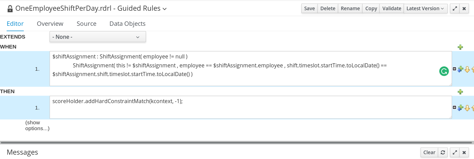
The OneEmployeeShiftPerDay guided rule creates a hard constraint that employees are not assigned more than one shift per day. In the employee rostering example, this constraint is created using the guided rule designer.
Procedure
- In Business Central, go to Menu → Design → Projects and click the project name.
- Click Add Asset → Guided Rule.
-
Enter
OneEmployeeShiftPerDayas the Guided Rule name and select theemployeerostering.employeerosteringPackage. - Click Ok to create the rule asset.
-
Add a WHEN condition by clicking the
in the WHEN field.
- Select Free form DRL from the Add a condition to the rule window.
In the free form DRL box, type the following condition:
$shiftAssignment : ShiftAssignment( employee != null )
		ShiftAssignment( this != $shiftAssignment , employee == $shiftAssignment.employee , shift.timeslot.startTime.toLocalDate() == $shiftAssignment.shift.timeslot.startTime.toLocalDate() )
This condition states that a shift cannot be assigned to an employee that already has another shift assignment on the same day.
-
Add the THEN condition by clicking the
in the THEN field.
- Select Add free form DRL from the Add a new action window.
In the free form DRL box, type the following condition:
scoreHolder.addHardConstraintMatch(kcontext, -1);
- Click Validate in the upper-right corner to check all rule conditions are valid. If the rule validation fails, address any problems described in the error message, review all components in the rule, and try again to validate the rule until the rule passes.
- Click Save to save the rule.
For more information about creating guided rules, see Designing a decision service using guided rules.
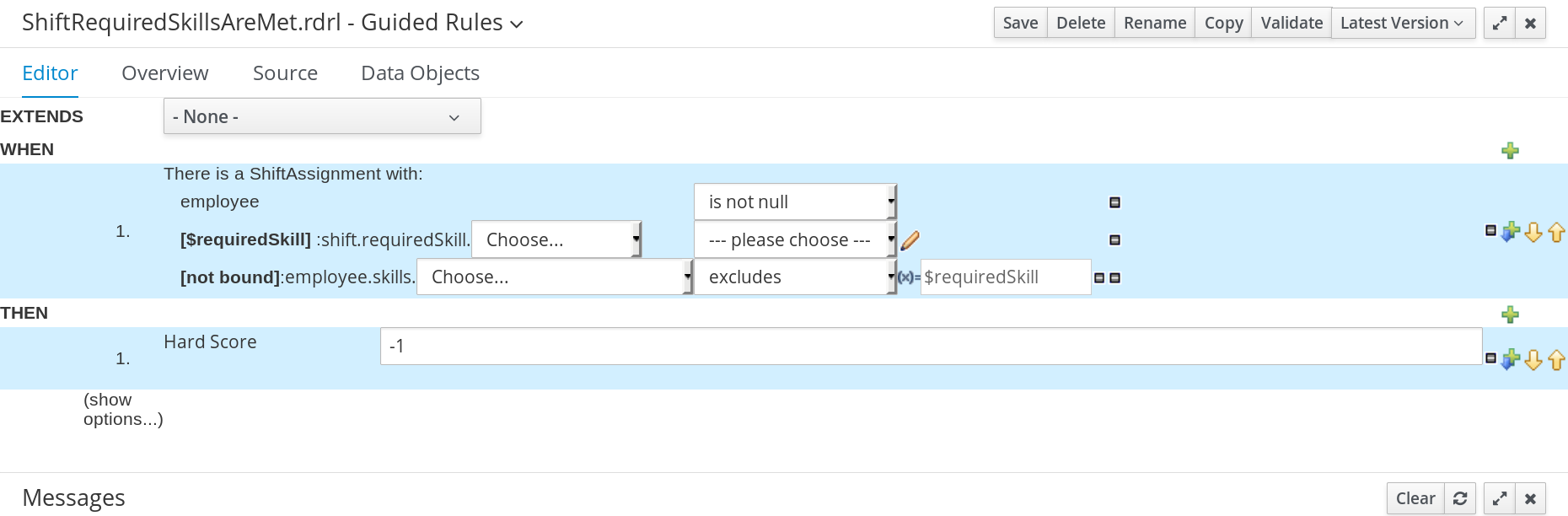
2.2.5.4. Creating a guided rule to match skills to shift requirements
The ShiftReqiredSkillsAreMet guided rule creates a hard constraint that ensures all shifts are assigned an employee with the correct set of skills. In the employee rostering example, this constraint is created using the guided rule designer.
Procedure
- In Business Central, go to Menu → Design → Projects and click the project name.
- Click Add Asset → Guided Rule.
-
Enter
ShiftReqiredSkillsAreMetas the Guided Rule name and select theemployeerostering.employeerosteringPackage. - Click Ok to create the rule asset.
-
Add a WHEN condition by clicking the
in the WHEN field.
-
Select
ShiftAssignmentin the Add a condition to the rule window. Click +Ok. -
Click the
ShiftAssignmentcondition, and selectemployeefrom the Add a restriction on a field drop-down list. -
In the designer, click the drop-down list next to
employeeand selectis not null. Click the
ShiftAssignmentcondition, and click Expression editor.-
In the designer, click
[not bound]to open the Expression editor, and bind the expression to the variable$requiredSkill. Click Set. -
In the designer, next to
$requiredSkill, selectshiftfrom the first drop-down list, thenrequiredSkillfrom the next drop-down list.
-
In the designer, click
Click the
ShiftAssignmentcondition, and click Expression editor.-
In the designer, next to
[not bound], selectemployeefrom the first drop-down list, thenskillsfrom the next drop-down list. -
Leave the next drop-down list as
Choose. -
In the next drop-down box, change
please choosetoexcludes. -
Click the
icon next to
excludes, and in the Field value window, click the New formula button. -
Type
$requiredSkillinto the formula box.
-
In the designer, next to
-
Add the THEN condition by clicking the
in the THEN field.
-
Select
Modify Hard Scorein the Add a new action window. Click +Ok. -
Type
-1into the score actions box. - Click Validate in the upper-right corner to check all rule conditions are valid. If the rule validation fails, address any problems described in the error message, review all components in the rule, and try again to validate the rule until the rule passes.
- Click Save to save the rule.
For more information about creating guided rules, see Designing a decision service using guided rules.
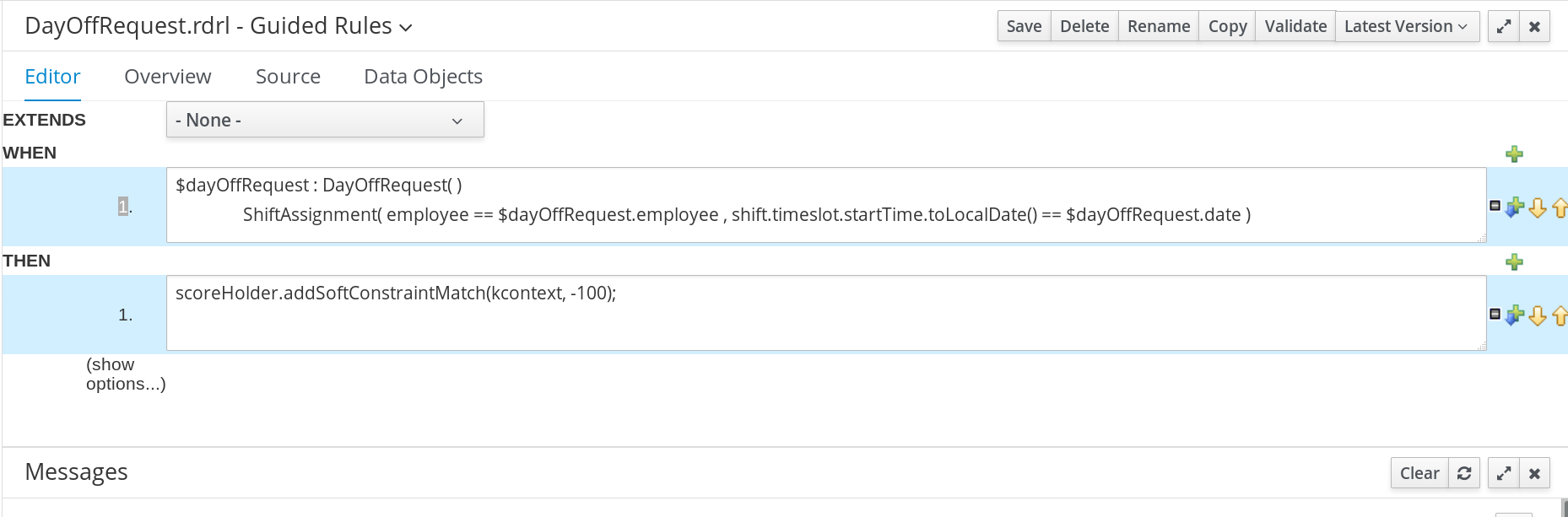
2.2.5.5. Creating a guided rule to manage day off requests
The DayOffRequest guided rule creates a soft constraint. This constraint allows a shift to be reassigned to another employee in the event the employee who was originally assigned the shift is no longer able to work that day. In the employee rostering example, this constraint is created using the guided rule designer.
Procedure
- In Business Central, go to Menu → Design → Projects and click the project name.
- Click Add Asset → Guided Rule.
-
Enter
DayOffRequestas the Guided Rule name and select theemployeerostering.employeerosteringPackage. - Click Ok to create the rule asset.
-
Add a WHEN condition by clicking the
in the WHEN field.
- Select Free form DRL from the Add a condition to the rule window.
In the free form DRL box, type the following condition:
$dayOffRequest : DayOffRequest( )
		ShiftAssignment( employee == $dayOffRequest.employee , shift.timeslot.startTime.toLocalDate() == $dayOffRequest.date )
This condition states if a shift is assigned to an employee who has made a day off request, the employee can be unassigned the shift on that day.
-
Add the THEN condition by clicking the
in the THEN field.
- Select Add free form DRL from the Add a new action window.
In the free form DRL box, type the following condition:
scoreHolder.addSoftConstraintMatch(kcontext, -100);
- Click Validate in the upper-right corner to check all rule conditions are valid. If the rule validation fails, address any problems described in the error message, review all components in the rule, and try again to validate the rule until the rule passes.
- Click Save to save the rule.
For more information about creating guided rules, see Designing a decision service using guided rules.
2.2.6. Creating a solver configuration for employee rostering
You can create and edit Solver configurations in Business Central. The Solver configuration designer creates a solver configuration that can be run after the project is deployed.
Prerequisites
- Red Hat Process Automation Manager has been downloaded and installed.
- You have created and configured all of the relevant assets for the employee rostering example.
Procedure
- In Business Central, click Menu → Projects, and click your project to open it.
- In the Assets perspective, click Add Asset → Solver configuration
In the Create new Solver configuration window, type the name
EmployeeRosteringSolverConfigfor your Solver and click Ok.This opens the Solver configuration designer.
In the Score Director Factory configuration section, define a KIE base that contains scoring rule definitions. The employee rostering sample project uses
defaultKieBase.-
Select one of the KIE sessions defined within the KIE base. The employee rostering sample project uses
defaultKieSession.
-
Select one of the KIE sessions defined within the KIE base. The employee rostering sample project uses
- Click Validate in the upper-right corner to check the Score Director Factory configuration is correct. If validation fails, address any problems described in the error message, and try again to validate until the configuration passes.
- Click Save to save the Solver configuration.
2.2.7. Configuring Solver termination for the employee rostering project
You can configure the Solver to terminate after a specified amount of time. By default, the planning engine is given an unlimited time period to solve a problem instance.
The employee rostering sample project is set up to run for 30 seconds.
Prerequisites
-
You have created all relevant assets for the employee rostering project and created the
EmployeeRosteringSolverConfigsolver configuration in Business Central as described in Section 2.2.6, “Creating a solver configuration for employee rostering”.
Procedure
-
Open the
EmployeeRosteringSolverConfigfrom the Assets perspective. This will open the Solver configuration designer. - In the Termination section, click Add to create new termination element within the selected logical group.
-
Select the
Time spenttermination type from the drop-down list. This is added as an input field in the termination configuration. - Use the arrows next to the time elements to adjust the amount of time spent to 30 seconds.
- Click Validate in the upper-right corner to check the Score Director Factory configuration is correct. If validation fails, address any problems described in the error message, and try again to validate until the configuration passes.
- Click Save to save the Solver configuration.
2.3. Accessing the solver using the REST API
After deploying or re-creating the sample solver, you can access it using the REST API.
You must register a solver instance using the REST API. Then you can supply data sets and retrieve optimized solutions.
Prerequisites
- The employee rostering project is set up and deployed according to the previous sections in this document. You can either deploy the sample project, as described in Section 2.1, “Deploying the employee rostering sample project in Business Central”, or re-create the project, as described in Section 2.2, “Re-creating the employee rostering sample project”.
2.3.1. Registering the Solver using the REST API
You must register the solver instance using the REST API before you can use the solver.
Each solver instance is capable of optimizing one planning problem at a time.
Procedure
Create a HTTP request using the following header:
authorization: admin:admin
X-KIE-ContentType: xstream
content-type: application/xml
Register the Solver using the following request:
- PUT
-
http://localhost:8080/kie-server/services/rest/server/containers/employeerostering_1.0.0-SNAPSHOT/solvers/EmployeeRosteringSolver - Request body
<solver-instance>
  <solver-config-file>employeerostering/employeerostering/EmployeeRosteringSolverConfig.solver.xml</solver-config-file>
</solver-instance>
2.3.2. Calling the Solver using the REST API
After registering the solver instance, you can use the REST API to submit a data set to the solver and to retrieve an optimized solution.
Procedure
Create a HTTP request using the following header:
authorization: admin:admin
X-KIE-ContentType: xstream
content-type: application/xml
Submit a request to the Solver with a data set, as in the following example:
- POST
-
http://localhost:8080/kie-server/services/rest/server/containers/employeerostering_1.0.0-SNAPSHOT/solvers/EmployeeRosteringSolver/state/solving - Request body
<employeerostering.employeerostering.EmployeeRoster>
  <employeeList>
    <employeerostering.employeerostering.Employee>
      <name>John</name>
      <skills>
        <employeerostering.employeerostering.Skill>
          <name>reading</name>
        </employeerostering.employeerostering.Skill>
      </skills>
    </employeerostering.employeerostering.Employee>
    <employeerostering.employeerostering.Employee>
      <name>Mary</name>
      <skills>
        <employeerostering.employeerostering.Skill>
          <name>writing</name>
        </employeerostering.employeerostering.Skill>
      </skills>
    </employeerostering.employeerostering.Employee>
    <employeerostering.employeerostering.Employee>
      <name>Petr</name>
      <skills>
        <employeerostering.employeerostering.Skill>
          <name>speaking</name>
        </employeerostering.employeerostering.Skill>
      </skills>
    </employeerostering.employeerostering.Employee>
  </employeeList>
  <shiftList>
    <employeerostering.employeerostering.Shift>
      <timeslot>
        <startTime>2017-01-01T00:00:00</startTime>
        <endTime>2017-01-01T01:00:00</endTime>
      </timeslot>
      <requiredSkill reference="../../../employeeList/employeerostering.employeerostering.Employee/skills/employeerostering.employeerostering.Skill"/>
    </employeerostering.employeerostering.Shift>
    <employeerostering.employeerostering.Shift>
      <timeslot reference="../../employeerostering.employeerostering.Shift/timeslot"/>
      <requiredSkill reference="../../../employeeList/employeerostering.employeerostering.Employee[3]/skills/employeerostering.employeerostering.Skill"/>
    </employeerostering.employeerostering.Shift>
    <employeerostering.employeerostering.Shift>
      <timeslot reference="../../employeerostering.employeerostering.Shift/timeslot"/>
      <requiredSkill reference="../../../employeeList/employeerostering.employeerostering.Employee[2]/skills/employeerostering.employeerostering.Skill"/>
    </employeerostering.employeerostering.Shift>
  </shiftList>
  <skillList>
    <employeerostering.employeerostering.Skill reference="../../employeeList/employeerostering.employeerostering.Employee/skills/employeerostering.employeerostering.Skill"/>
    <employeerostering.employeerostering.Skill reference="../../employeeList/employeerostering.employeerostering.Employee[3]/skills/employeerostering.employeerostering.Skill"/>
    <employeerostering.employeerostering.Skill reference="../../employeeList/employeerostering.employeerostering.Employee[2]/skills/employeerostering.employeerostering.Skill"/>
  </skillList>
  <timeslotList>
    <employeerostering.employeerostering.Timeslot reference="../../shiftList/employeerostering.employeerostering.Shift/timeslot"/>
  </timeslotList>
  <dayOffRequestList/>
  <shiftAssignmentList>
    <employeerostering.employeerostering.ShiftAssignment>
      <shift reference="../../../shiftList/employeerostering.employeerostering.Shift"/>
    </employeerostering.employeerostering.ShiftAssignment>
    <employeerostering.employeerostering.ShiftAssignment>
      <shift reference="../../../shiftList/employeerostering.employeerostering.Shift[3]"/>
    </employeerostering.employeerostering.ShiftAssignment>
    <employeerostering.employeerostering.ShiftAssignment>
      <shift reference="../../../shiftList/employeerostering.employeerostering.Shift[2]"/>
    </employeerostering.employeerostering.ShiftAssignment>
  </shiftAssignmentList>
</employeerostering.employeerostering.EmployeeRoster>
Request the best solution to the planning problem:
- GET
http://localhost:8080/kie-server/services/rest/server/containers/employeerostering_1.0.0-SNAPSHOT/solvers/EmployeeRosteringSolver/bestsolutionExample response
<solver-instance>
  <container-id>employee-rostering</container-id>
  <solver-id>solver1</solver-id>
  <solver-config-file>employeerostering/employeerostering/EmployeeRosteringSolverConfig.solver.xml</solver-config-file>
  <status>NOT_SOLVING</status>
  <score scoreClass="org.optaplanner.core.api.score.buildin.hardsoft.HardSoftScore">0hard/0soft</score>
  <best-solution class="employeerostering.employeerostering.EmployeeRoster">
    <employeeList>
      <employeerostering.employeerostering.Employee>
        <name>John</name>
        <skills>
          <employeerostering.employeerostering.Skill>
            <name>reading</name>
          </employeerostering.employeerostering.Skill>
        </skills>
      </employeerostering.employeerostering.Employee>
      <employeerostering.employeerostering.Employee>
        <name>Mary</name>
        <skills>
          <employeerostering.employeerostering.Skill>
            <name>writing</name>
          </employeerostering.employeerostering.Skill>
        </skills>
      </employeerostering.employeerostering.Employee>
      <employeerostering.employeerostering.Employee>
        <name>Petr</name>
        <skills>
          <employeerostering.employeerostering.Skill>
            <name>speaking</name>
          </employeerostering.employeerostering.Skill>
        </skills>
      </employeerostering.employeerostering.Employee>
    </employeeList>
    <shiftList>
      <employeerostering.employeerostering.Shift>
        <timeslot>
          <startTime>2017-01-01T00:00:00</startTime>
          <endTime>2017-01-01T01:00:00</endTime>
        </timeslot>
        <requiredSkill reference="../../../employeeList/employeerostering.employeerostering.Employee/skills/employeerostering.employeerostering.Skill"/>
      </employeerostering.employeerostering.Shift>
      <employeerostering.employeerostering.Shift>
        <timeslot reference="../../employeerostering.employeerostering.Shift/timeslot"/>
        <requiredSkill reference="../../../employeeList/employeerostering.employeerostering.Employee[3]/skills/employeerostering.employeerostering.Skill"/>
      </employeerostering.employeerostering.Shift>
      <employeerostering.employeerostering.Shift>
        <timeslot reference="../../employeerostering.employeerostering.Shift/timeslot"/>
        <requiredSkill reference="../../../employeeList/employeerostering.employeerostering.Employee[2]/skills/employeerostering.employeerostering.Skill"/>
      </employeerostering.employeerostering.Shift>
    </shiftList>
    <skillList>
      <employeerostering.employeerostering.Skill reference="../../employeeList/employeerostering.employeerostering.Employee/skills/employeerostering.employeerostering.Skill"/>
      <employeerostering.employeerostering.Skill reference="../../employeeList/employeerostering.employeerostering.Employee[3]/skills/employeerostering.employeerostering.Skill"/>
      <employeerostering.employeerostering.Skill reference="../../employeeList/employeerostering.employeerostering.Employee[2]/skills/employeerostering.employeerostering.Skill"/>
    </skillList>
    <timeslotList>
      <employeerostering.employeerostering.Timeslot reference="../../shiftList/employeerostering.employeerostering.Shift/timeslot"/>
    </timeslotList>
    <dayOffRequestList/>
    <shiftAssignmentList/>
    <score>0hard/0soft</score>
  </best-solution>
</solver-instance>
Chapter 3. Getting started with Java solvers: A cloud balancing example
An example demonstrates development of a basic Red Hat Business Optimizer solver using Java code.
Suppose your company owns a number of cloud computers and needs to run a number of processes on those computers. You must assign each process to a computer.
The following hard constraints must be fulfilled:
Every computer must be able to handle the minimum hardware requirements of the sum of its processes:
- CPU capacity: The CPU power of a computer must be at least the sum of the CPU power required by the processes assigned to that computer.
- Memory capacity: The RAM memory of a computer must be at least the sum of the RAM memory required by the processes assigned to that computer.
- Network capacity: The network bandwidth of a computer must be at least the sum of the network bandwidth required by the processes assigned to that computer.
The following soft constraints should be optimized:
Each computer that has one or more processes assigned incurs a maintenance cost (which is fixed per computer).
- Cost: Minimize the total maintenance cost.
This problem is a form of bin packing. In the following simplified example, we assign four processes to two computers with two constraints (CPU and RAM) with a simple algorithm:
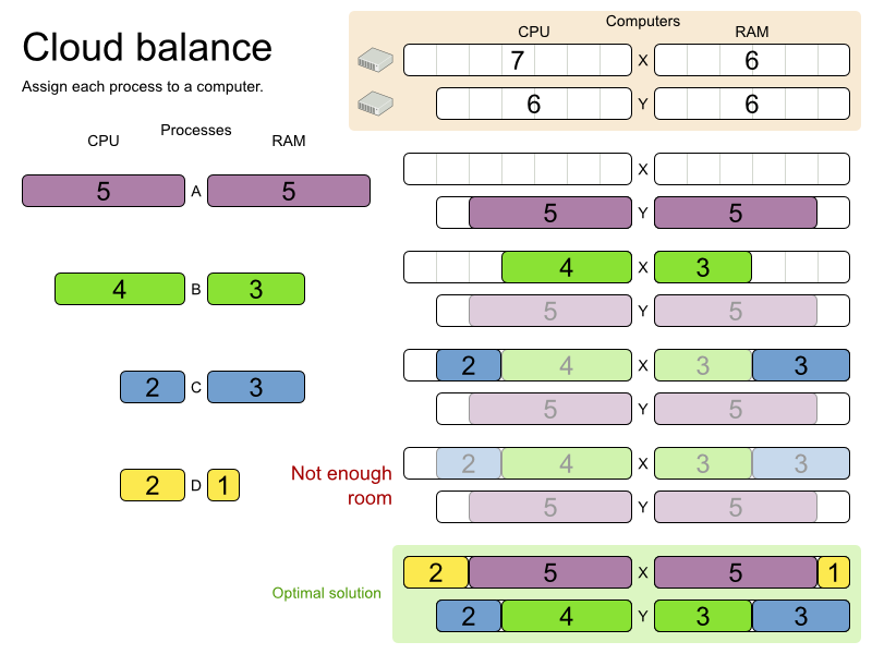
The simple algorithm used here is the First Fit Decreasing algorithm, which assigns the bigger processes first and assigns the smaller processes to the remaining space. As you can see, it is not optimal, as it does not leave enough room to assign the yellow process D.
Business Optimizer finds a more optimal solution by using additional, smarter algorithms. It also scales: both in data (more processes, more computers) and constraints (more hardware requirements, other constraints).
The following summary applies to this example, as well as to an advanced implementation with more constraints that is described in Section 4.10, “Machine reassignment (Google ROADEF 2012)”:
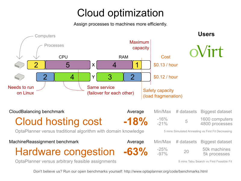
Table 3.1. Cloud balancing problem size
| Problem size | Computers | Processes | Search space |
|---|---|---|---|
| 2computers-6processes | 2 | 6 | 64 |
| 3computers-9processes | 3 | 9 | 10^4 |
| 4computers-012processes | 4 | 12 | 10^7 |
| 100computers-300processes | 100 | 300 | 10^600 |
| 200computers-600processes | 200 | 600 | 10^1380 |
| 400computers-1200processes | 400 | 1200 | 10^3122 |
| 800computers-2400processes | 800 | 2400 | 10^6967 |
3.1. Domain Model Design
Using a domain model helps determine which classes are planning entities and which of their properties are planning variables. It also helps to simplify constraints, improve performance, and increase flexibility for future needs.
3.1.1. Designing a domain model
To create a domain model, define all the objects that represent the input data for the problem. In this example, the objects are processes and computers.
A separate object in the domain model must represent a full data set of the problem, which contains the input data as well as a solution. In this example, this object holds a list of computers and a list of processes. Each process is assigned to a computer; the distribution of processes between computers is the solution.
Procedure
- Draw a class diagram of your domain model.
- Normalize it to remove duplicate data.
Write down some sample instances for each class. Sample instances are entity properties that are relevant for planning purposes.
Computer: Represents a computer with certain hardware and maintenance costs.In this example, the sample instances for the
Computerclass arecpuPower,memory,networkBandwidth,cost.Process: Represents a process with a demand. Needs to be assigned to aComputerby Planner.Sample instances for
ProcessarerequiredCpuPower,requiredMemory, andrequiredNetworkBandwidth.CloudBalance: Represents the distribution of processes between computers. Contains everyComputerandProcessfor a certain data set.For an object representing the full data set and solution, a sample instance holding the score must be present. Business Optimizer can calculate and compare the scores for different solutions; the solution with the highest score is the optimal solution. Therefore, the sample instance for
CloudBalanceisscore.
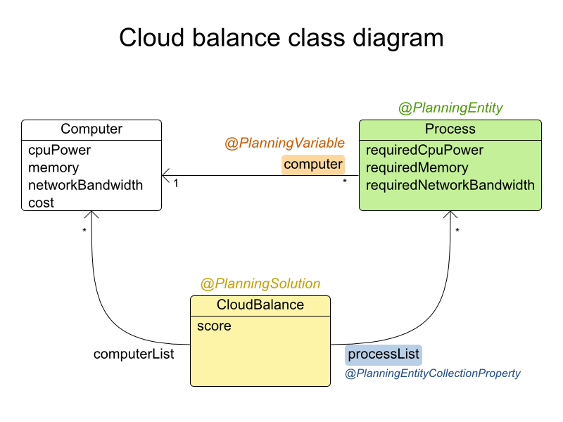
Determine which relationships (or fields) change during planning:
Planning entity: The class (or classes) that Business Optimizer can change during solving. In this example, it is the class
Process, because we can move processes to different computers.- A class representing input data that Business Optimizer can not change is known as a problem fact.
-
Planning variable: The property (or properties) of a planning entity class that changes during solving. In this example, it is the property
computeron the classProcess. -
Planning solution: The class that represents a solution to the problem. This class must represent the full data set and contain all planning entities. In this example that is the class
CloudBalance.
In the UML class diagram below, the Business Optimizer concepts are already annotated:
You can find the class definitions for this example in the examples/sources/src/main/java/org/optaplanner/examples/cloudbalancing/domain directory.
3.1.2. The Computer Class
The Computer class is a Java object that stores data, sometimes known as a POJO (Plain Old Java Object). Usually, you will have more of this kind of classes with input data.
Example 3.1. CloudComputer.java
public class CloudComputer ... {

    private int cpuPower;
    private int memory;
    private int networkBandwidth;
    private int cost;

    ... // getters
}
3.1.3. The Process Class
The Process class is the class that is modified during solving.
We need to tell Business Optimizer that it can change the property computer. To do this, annotate the class with @PlanningEntity and annotate the getComputer() getter with @PlanningVariable.
Of course, the property computer needs a setter too, so Business Optimizer can change it during solving.
Example 3.2. CloudProcess.java
@PlanningEntity(...)
public class CloudProcess ... {

    private int requiredCpuPower;
    private int requiredMemory;
    private int requiredNetworkBandwidth;

    private CloudComputer computer;

    ... // getters

    @PlanningVariable(valueRangeProviderRefs = {"computerRange"})
    public CloudComputer getComputer() {
        return computer;
    }

    public void setComputer(CloudComputer computer) {
        computer = computer;
    }

    // ************************************************************************
    // Complex methods
    // ************************************************************************

    ...

}
Business Optimizer needs to know which values it can choose from to assign to the property computer. Those values are retrieved from the method CloudBalance.getComputerList() on the planning solution, which returns a list of all computers in the current data set.
The @PlanningVariable's valueRangeProviderRefs parameter on CloudProcess.getComputer() needs to match with the @ValueRangeProvider's id on CloudBalance.getComputerList().
You can also use annotations on fields instead of getters.
3.1.4. The CloudBalance Class
The CloudBalance class has a @PlanningSolution annotation.
This class holds a list of all computers and processes. It represents both the planning problem and (if it is initialized) the planning solution.
The CloudBalance class has the following key attributes:
It holds a collection of processes that Business Optimizer can change. We annotate the getter
getProcessList()with@PlanningEntityCollectionProperty, so that Business Optimizer can retrieve the processes that it can change. To save a solution, Business Optimizer initializes a new instance of the class with the list of changed processes.-
It also has a
@PlanningScoreannotated propertyscore, which is theScoreof that solution in its current state. Business Optimizer automatically updates it when it calculates aScorefor a solution instance; therefore, this property needs a setter. -
Especially for score calculation with Drools, the property
computerListneeds to be annotated with a@ProblemFactCollectionPropertyso that Business Optimizer can retrieve a list of computers (problem facts) and make it available to the decision engine.
-
It also has a
Example 3.3. CloudBalance.java
@PlanningSolution
public class CloudBalance ... {

    private List<CloudComputer> computerList;

    private List<CloudProcess> processList;

    private HardSoftScore score;

    @ValueRangeProvider(id = "computerRange")
    @ProblemFactCollectionProperty
    public List<CloudComputer> getComputerList() {
        return computerList;
    }

    @PlanningEntityCollectionProperty
    public List<CloudProcess> getProcessList() {
        return processList;
    }

    @PlanningScore
    public HardSoftScore getScore() {
        return score;
    }

    public void setScore(HardSoftScore score) {
        this.score = score;
    }

    ...
}
3.2. Running the Cloud Balancing Hello World
You can run a sample "hello world" application to demonstrate the solver.
Procedure
- Download and configure the examples in your preferred IDE. For instructions on downloading and configuring examples in an IDE, see Section 4.1.3, “Running the Red Hat Business Optimizer examples in an IDE (IntelliJ, Eclipse, or Netbeans)”.
Create a run configuration with the following main class:
org.optaplanner.examples.cloudbalancing.app.CloudBalancingHelloWorldBy default, the Cloud Balancing Hello World is configured to run for 120 seconds.
Result
The application executes the following code:
Example 3.4. CloudBalancingHelloWorld.java
public class CloudBalancingHelloWorld {

    public static void main(String[] args) {
        // Build the Solver
        SolverFactory<CloudBalance> solverFactory = SolverFactory.createFromXmlResource("org/optaplanner/examples/cloudbalancing/solver/cloudBalancingSolverConfig.xml");
        Solver<CloudBalance> solver = solverFactory.buildSolver();

        // Load a problem with 400 computers and 1200 processes
        CloudBalance unsolvedCloudBalance = new CloudBalancingGenerator().createCloudBalance(400, 1200);

        // Solve the problem
        CloudBalance solvedCloudBalance = solver.solve(unsolvedCloudBalance);

        // Display the result
        System.out.println("\nSolved cloudBalance with 400 computers and 1200 processes:\n" + toDisplayString(solvedCloudBalance));
    }

    ...
}
The code example does the following:
Build the
Solverbased on a solver configuration (in this case an XML file,cloudBalancingSolverConfig.xml, from the classpath).Building the
Solveris the most complicated part of this procedure. For more details, see Section 3.3, “Solver Configuration”.SolverFactory<CloudBalance> solverFactory = SolverFactory.createFromXmlResource( "org/optaplanner/examples/cloudbalancing/solver/cloudBalancingSolverConfig.xml"); Solver solver<CloudBalance> = solverFactory.buildSolver();Load the problem.
CloudBalancingGeneratorgenerates a random problem: you will replace this with a class that loads a real problem, for example from a database.CloudBalance unsolvedCloudBalance = new CloudBalancingGenerator().createCloudBalance(400, 1200);
Solve the problem.
CloudBalance solvedCloudBalance = solver.solve(unsolvedCloudBalance);
Display the result.
        System.out.println("\nSolved cloudBalance with 400 computers and 1200 processes:\n"
                + toDisplayString(solvedCloudBalance));
3.3. Solver Configuration
The solver configuration file determines how the solving process works; it is considered a part of the code. The file is named examples/sources/src/main/resources/org/optaplanner/examples/cloudbalancing/solver/cloudBalancingSolverConfig.xml.
Example 3.5. cloudBalancingSolverConfig.xml
<?xml version="1.0" encoding="UTF-8"?>
<solver>
  <!-- Domain model configuration -->
  <scanAnnotatedClasses/>

  <!-- Score configuration -->
  <scoreDirectorFactory>
    <easyScoreCalculatorClass>org.optaplanner.examples.cloudbalancing.optional.score.CloudBalancingEasyScoreCalculator</easyScoreCalculatorClass>
    <!--<scoreDrl>org/optaplanner/examples/cloudbalancing/solver/cloudBalancingScoreRules.drl</scoreDrl>-->
  </scoreDirectorFactory>

  <!-- Optimization algorithms configuration -->
  <termination>
    <secondsSpentLimit>30</secondsSpentLimit>
  </termination>
</solver>
This solver configuration consists of three parts:
Domain model configuration: What can Business Optimizer change?
We need to make Business Optimizer aware of our domain classes. In this configuration, it will automatically scan all classes in your classpath (for a
@PlanningEntityor@PlanningSolutionannotation):<scanAnnotatedClasses/>
Score configuration: How should Business Optimizer optimize the planning variables? What is our goal?
Since we have hard and soft constraints, we use a
HardSoftScore. But we need to tell Business Optimizer how to calculate the score, depending on our business requirements. Further down, we will look into two alternatives to calculate the score: using a basic Java implementation and using Drools DRL.<scoreDirectorFactory> <easyScoreCalculatorClass>org.optaplanner.examples.cloudbalancing.optional.score.CloudBalancingEasyScoreCalculator</easyScoreCalculatorClass> <!--<scoreDrl>org/optaplanner/examples/cloudbalancing/solver/cloudBalancingScoreRules.drl</scoreDrl>--> </scoreDirectorFactory>Optimization algorithms configuration: How should Business Optimizer optimize it? In this case, we use the default optimization algorithms (because no explicit optimization algorithms are configured) for 30 seconds:
  <termination>
    <secondsSpentLimit>30</secondsSpentLimit>
  </termination>
Business Optimizer should get a good result in seconds (and even in less than 15 milliseconds if the real-time planning feature is used), but the more time it has, the better the result will be. Advanced use cases might use different termination criteria than a hard time limit.
The default algorithms will already easily surpass human planners and most in-house implementations. You can use the advanced Benchmarker feature to power tweak to get even better results.
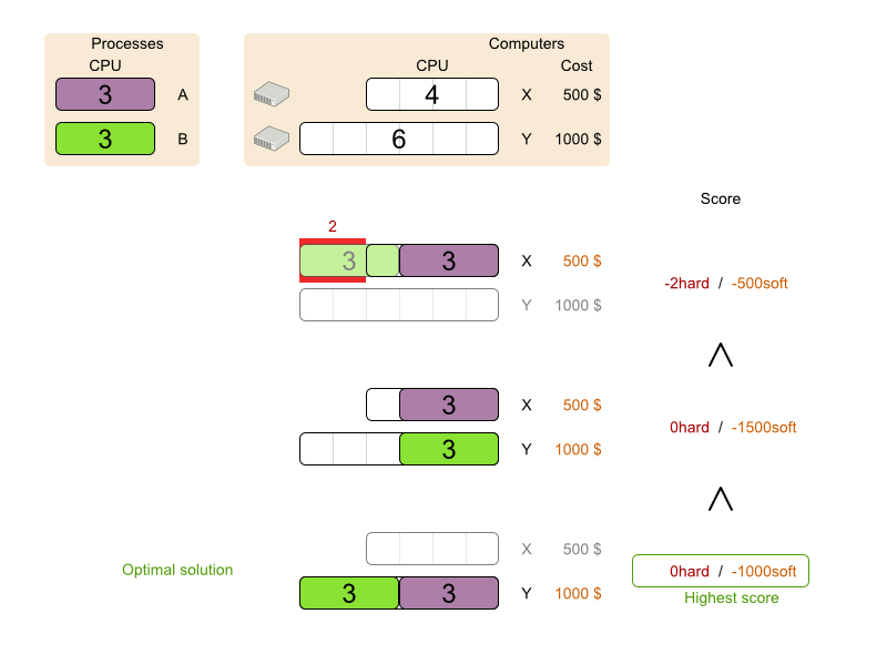
3.4. Score Configuration
Business Optimizer will search for the Solution with the highest Score. This example uses a HardSoftScore, which means Business Optimizer will look for the solution with no hard constraints broken (fulfill hardware requirements) and as little as possible soft constraints broken (minimize maintenance cost).
Of course, Business Optimizer needs to be told about these domain-specific score constraints. You can define constraints using the Java or Drools languages.
3.4.1. Configuring score calculation using Java
One way to define a score function is to implement the interface EasyScoreCalculator in plain Java.
Procedure
In the
cloudBalancingSolverConfig.xmlfile, add or uncomment the setting:<scoreDirectorFactory> <easyScoreCalculatorClass>org.optaplanner.examples.cloudbalancing.optional.score.CloudBalancingEasyScoreCalculator</easyScoreCalculatorClass> </scoreDirectorFactory>Implement the
calculateScore(Solution)method to return aHardSoftScoreinstance.Example 3.6. CloudBalancingEasyScoreCalculator.java
public class CloudBalancingEasyScoreCalculator implements EasyScoreCalculator<CloudBalance> {

    /**
     * A very simple implementation. The double loop can easily be removed by using Maps as shown in
     * {@link CloudBalancingMapBasedEasyScoreCalculator#calculateScore(CloudBalance)}.
     */
    public HardSoftScore calculateScore(CloudBalance cloudBalance) {
        int hardScore = 0;
        int softScore = 0;
        for (CloudComputer computer : cloudBalance.getComputerList()) {
            int cpuPowerUsage = 0;
            int memoryUsage = 0;
            int networkBandwidthUsage = 0;
            boolean used = false;

            // Calculate usage
            for (CloudProcess process : cloudBalance.getProcessList()) {
                if (computer.equals(process.getComputer())) {
                    cpuPowerUsage += process.getRequiredCpuPower();
                    memoryUsage += process.getRequiredMemory();
                    networkBandwidthUsage += process.getRequiredNetworkBandwidth();
                    used = true;
                }
            }

            // Hard constraints
            int cpuPowerAvailable = computer.getCpuPower() - cpuPowerUsage;
            if (cpuPowerAvailable < 0) {
                hardScore += cpuPowerAvailable;
            }
            int memoryAvailable = computer.getMemory() - memoryUsage;
            if (memoryAvailable < 0) {
                hardScore += memoryAvailable;
            }
            int networkBandwidthAvailable = computer.getNetworkBandwidth() - networkBandwidthUsage;
            if (networkBandwidthAvailable < 0) {
                hardScore += networkBandwidthAvailable;
            }

            // Soft constraints
            if (used) {
                softScore -= computer.getCost();
            }
        }
        return HardSoftScore.valueOf(hardScore, softScore);
    }

}
Even if we optimize the code above to use Maps to iterate through the processList only once, it is still slow because it does not do incremental score calculation.
To fix that, either use incremental Java score calculation or Drools score calculation. Incremental Java score calculation is not covered in this guide.
3.4.2. Configuring score calculation using Drools
You can use Drools rule language (DRL) to define constraints. Drools score calculation uses incremental calculation, where every score constraint is written as one or more score rules.
Using the decision engine for score calculation enables you to integrate with other Drools technologies, such as decision tables (XLS or web based), Business Central, and other supported features.
Procedure
Add a
scoreDrlresource in the classpath to use the decision engine as a score function. In thecloudBalancingSolverConfig.xmlfile, add or uncomment the setting:<scoreDirectorFactory> <scoreDrl>org/optaplanner/examples/cloudbalancing/solver/cloudBalancingScoreRules.drl</scoreDrl> </scoreDirectorFactory>Create the hard constraints. These constraints ensure that all computers have enough CPU, RAM and network bandwidth to support all their processes:
Example 3.7. cloudBalancingScoreRules.drl - Hard Constraints
...

import org.optaplanner.examples.cloudbalancing.domain.CloudBalance;
import org.optaplanner.examples.cloudbalancing.domain.CloudComputer;
import org.optaplanner.examples.cloudbalancing.domain.CloudProcess;

global HardSoftScoreHolder scoreHolder;

// ############################################################################
// Hard constraints
// ############################################################################

rule "requiredCpuPowerTotal"
    when
        $computer : CloudComputer($cpuPower : cpuPower)
        accumulate(
            CloudProcess(
                computer == $computer,
                $requiredCpuPower : requiredCpuPower);
            $requiredCpuPowerTotal : sum($requiredCpuPower);
            $requiredCpuPowerTotal > $cpuPower
        )
    then
        scoreHolder.addHardConstraintMatch(kcontext, $cpuPower - $requiredCpuPowerTotal);
end

rule "requiredMemoryTotal"
    ...
end

rule "requiredNetworkBandwidthTotal"
    ...
end
Create a soft constraint. This constraint minimizes the maintenance cost. It is applied only if hard constraints are met:
Example 3.8. cloudBalancingScoreRules.drl - Soft Constraints
// ############################################################################
// Soft constraints
// ############################################################################

rule "computerCost"
    when
        $computer : CloudComputer($cost : cost)
        exists CloudProcess(computer == $computer)
    then
        scoreHolder.addSoftConstraintMatch(kcontext, - $cost);
end
3.5. Further development of the solver
Now that this example works, you can try developing it further. For example, you can enrich the domain model and add extra constraints such as these:
-
Each
Processbelongs to aService. A computer might crash, so processes running the same service should (or must) be assigned to different computers. -
Each
Computeris located in aBuilding. A building might burn down, so processes of the same services should (or must) be assigned to computers in different buildings.
Chapter 4. Examples provided with Red Hat Business Optimizer
Several Red Hat Business Optimizer examples are shipped with Red Hat Process Automation Manager. You can review the code for examples and modify it as necessary to suit your needs.
Red Hat does not provide support for the example code included in the Red Hat Process Automation Manager distribution.
4.1. Downloading and running the examples
You can download the Red Hat Business Optimizer examples from the Red Hat Software Downloads website and run them.
4.1.1. Downloading Red Hat Business Optimizer examples
You can download the examples as a part of the Red Hat Process Automation Manager add-ons package.
Procedure
-
Download the
rhpam-7.10.0-add-ons.zipfile from the Software Downloads page. - Decompress the file.
-
Decompress the
rhpam-7.10-planner-engine.zipfile from the decompressed directory.
Result
In the decompressed rhpam-7.10-planner-engine directory, you can find example source code under the following subdirectories: * examples/sources/src/main/java/org/optaplanner/examples * examples/sources/src/main/resources/org/optaplanner/examples * webexamples/sources/src/main/java/org/optaplanner/examples * webexamples/sources/src/main/resources/org/optaplanner/examples
The table of examples in Section 4.2, “Table of Business Optimizer examples” lists directory names that are used for individual examples.
4.1.2. Running Business Optimizer examples
Red Hat Business Optimizer includes a number of examples to demonstrate a variety of use cases.
Prerequisites
- You have downloaded and decompressed the examples. For instructions about these actions, see Section 4.1.1, “Downloading Red Hat Business Optimizer examples”.
Procedure
In the
rhpam-7.10.0-planner-enginefolder, open theexamplesdirectory and use the appropriate script to run the examples:Linux or Mac:
$ cd examples
$ ./runExamples.sh
Windows:
$ cd examples
$ runExamples.bat
Select and run an example from the GUI application window:
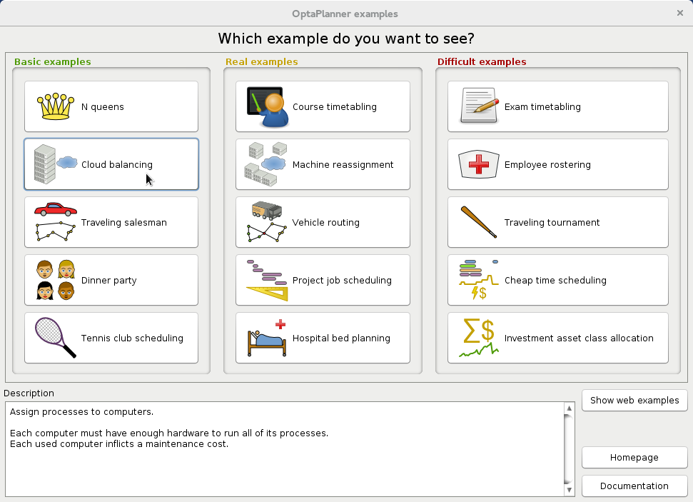
Red Hat Business Optimizer itself has no GUI dependencies. It runs just as well on a server or a mobile JVM as it does on the desktop.
4.1.3. Running the Red Hat Business Optimizer examples in an IDE (IntelliJ, Eclipse, or Netbeans)
If you use an integrated development environment (IDE), such as IntelliJ, Eclipse, or Netbeans, you can run your downloaded Red Hat Business Optimizer examples within your development environment.
Prerequisites
- You have downloaded and extracted the examples. For instructions about these actions, see Section 4.1.1, “Downloading Red Hat Business Optimizer examples”.
Procedure
Open the Red Hat Business Optimizer examples as a new project:
-
For IntelliJ or Netbeans, open
examples/sources/pom.xmlas the new project. The Maven integration guides you through the rest of the installation; skip the rest of the steps in this procedure. -
For Eclipse, open a new project for the directory
examples/sources.
-
For IntelliJ or Netbeans, open
-
Add all the JARs to the classpath from the directory
binariesand the directoryexamples/binaries, except for theexamples/binaries/optaplanner-examples-*.jarfile. -
Add the Java source directory
src/main/javaand the Java resources directorysrc/main/resources. Create a run configuration:
-
Main class:
org.optaplanner.examples.app.OptaPlannerExamplesApp -
VM parameters (optional):
-Xmx512M -server -Dorg.optaplanner.examples.dataDir=examples/sources/data -
Working directory:
examples/sources
-
Main class:
- Run the run configuration.
4.1.4. Running the web examples
Besides the GUI examples, Red Hat Process Automation Manager also includes a set of web examples for Red Hat Business Optimizer. The web examples include:
- Vehicle routing: Calculating the shortest possible route to pick up all items required for a number of different customers using either Leaflet or Google Maps visualizations.
- Cloud balancing: Assigning processes across computers with different specifications and costs.
Prerequisites
- You have downloaded and extracted the Red Hat Business Optimizer examples from the Red Hat Process Automation Manager add-ons package. For instructions, see Section 4.1.1, “Downloading Red Hat Business Optimizer examples”.
The web examples require several JEE APIs to run, such as the following APIs:
- Servlet
- JAX-RS
- CDI
These APIs are not required for Business Optimizer itself.
Procedure
- Download a JEE application server, such as JBoss EAP or WildFly and unzip it.
In the decompressed
rhpam-7.10.0-planner-enginedirectory, open the subdirectorywebexamples/binariesand deploy theoptaplanner-webexamples-*.warfile on the JEE application server.If using JBoss EAP in standalone mode, this can be done by adding the
optaplanner-webexamples-*.warfile to theJBOSS_home/standalone/deploymentsfolder.- Open the following address in a web browser: http://localhost:8080/optaplanner-webexamples/.
4.2. Table of Business Optimizer examples
Some of the Business Optimizer examples solve problems that are presented in academic contests. The Contest column in the following table lists the contests. It also identifies an example as being either realistic or unrealistic for the purpose of a contest. A realistic contest is an official, independent contest:
A realistic contest is an official, independent contest that meets the following standards:
- Clearly defined real-world use cases
- Real-world constraints
- Multiple real-world datasets
- Reproducible results within a specific time limit on specific hardware
- Serious participation from the academic and/or enterprise Operations Research community.
Realistic contests provide an objective comparison of Business Optimizer with competitive software and academic research.
Table 4.1. Examples overview
| Example | Domain | Size | Contest | Directory name |
|---|---|---|---|---|
| 1 entity class (1 variable) |
Entity ⇐
Value ⇐
Search space ⇐ | Pointless (cheatable) |
| |
| 1 entity class (1 variable) |
Entity ⇐
Value ⇐
Search space ⇐ | No (Defined by us) |
| |
| 1 entity class (1 chained variable) |
Entity ⇐
Value ⇐
Search space ⇐ | Unrealistic TSP web |
| |
| 1 entity class (1 variable) |
Entity ⇐
Value ⇐
Search space ⇐ | Unrealistic |
| |
| 1 entity class (1 variable) |
Entity ⇐
Value ⇐
Search space ⇐ | No (Defined by us) |
| |
| 1 entity class (2 variables) |
Entity ⇐
Value ⇐
Search space ⇐ | No (Defined by us) |
| |
| 1 entity class (2 variables) |
Entity ⇐
Value ⇐
Search space ⇐ | Realistic ITC 2007 track 3 |
| |
| 1 entity class (1 variable) |
Entity ⇐
Value ⇐
Search space ⇐ | Nearly realistic ROADEF 2012 |
| |
| 1 entity class (1 chained variable) 1 shadow entity class (1 automatic shadow variable) |
Entity ⇐
Value ⇐
Search space ⇐ | Unrealistic VRP web |
| |
| Vehicle routing with time windows | All of Vehicle routing (1 shadow variable) |
Entity ⇐
Value ⇐
Search space ⇐ | Unrealistic VRP web |
|
| 1 entity class (2 variables) (1 shadow variable) |
Entity ⇐
Value ⇐
Search space ⇐ | Nearly realistic MISTA 2013 |
| |
| 1 entity class (1 chained variable) (1 shadow variable) 1 shadow entity class (1 automatic shadow variable) |
Entity ⇐
Value ⇐
Search space ⇐ | No Defined by us |
| |
| 2 entity classes (same hierarchy) (2 variables) |
Entity ⇐
Value ⇐
Search space ⇐ | Realistic ITC 2007 track 1 |
| |
| 1 entity class (1 variable) |
Entity ⇐
Value ⇐
Search space ⇐ | Realistic INRC 2010 |
| |
| 1 entity class (1 variable) |
Entity ⇐
Value ⇐
Search space ⇐ | Unrealistic TTP |
| |
| 1 entity class (2 variables) |
Entity ⇐
Value ⇐
Search space ⇐ | Nearly realistic ICON Energy |
| |
| 1 entity class (1 variable) |
Entity ⇐
Value =
Search space ⇐ | No Defined by us |
| |
| 1 entity class (2 variables) |
Entity ⇐
Value ⇐
Search space ⇐ | No Defined by us |
| |
| 1 entity class (1 chained variable) (4 shadow variables) 1 shadow entity class (1 automatic shadow variable) |
Entity ⇐
Value ⇐
Search space ⇐ | No Defined by us |
| |
| 1 entity class (1 variable) 1 shadow entity class (1 automatic shadow variable) |
Entity ⇐
Value ⇐
Search space ⇐ | No Defined by us |
|
4.3. N queens
Place n queens on a n sized chessboard so that no two queens can attack each other. The most common n queens puzzle is the eight queens puzzle, with n = 8:

Constraints:
- Use a chessboard of n columns and n rows.
- Place n queens on the chessboard.
- No two queens can attack each other. A queen can attack any other queen on the same horizontal, vertical or diagonal line.
This documentation heavily uses the four queens puzzle as the primary example.
A proposed solution could be:
Figure 4.1. A wrong solution for the Four queens puzzle
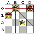
The above solution is wrong because queens A1 and B0 can attack each other (so can queens B0 and D0). Removing queen B0 would respect the "no two queens can attack each other" constraint, but would break the "place n queens" constraint.
Below is a correct solution:
Figure 4.2. A correct solution for the Four queens puzzle
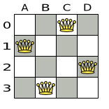
All the constraints have been met, so the solution is correct.
Note that most n queens puzzles have multiple correct solutions. We will focus on finding a single correct solution for a given n, not on finding the number of possible correct solutions for a given n.
Problem size
4queens   has   4 queens with a search space of    256.
8queens   has   8 queens with a search space of   10^7.
16queens  has  16 queens with a search space of  10^19.
32queens  has  32 queens with a search space of  10^48.
64queens  has  64 queens with a search space of 10^115.
256queens has 256 queens with a search space of 10^616.
The implementation of the n queens example has not been optimized because it functions as a beginner example. Nevertheless, it can easily handle 64 queens. With a few changes it has been shown to easily handle 5000 queens and more.
4.3.1. Domain model for N queens
This example uses the domain model to solve the four queens problem.
Creating a Domain Model
A good domain model will make it easier to understand and solve your planning problem.
This is the domain model for the n queens example:
public class Column {

    private int index;

    // ... getters and setters
}
public class Row { private int index; // ... getters and setters }public class Queen { private Column column; private Row row; public int getAscendingDiagonalIndex() {...} public int getDescendingDiagonalIndex() {...} // ... getters and setters }Calculating the Search Space.
A
Queeninstance has aColumn(for example: 0 is column A, 1 is column B, …) and aRow(its row, for example: 0 is row 0, 1 is row 1, …).The ascending diagonal line and the descending diagonal line can be calculated based on the column and the row.
The column and row indexes start from the upper left corner of the chessboard.
public class NQueens {

    private int n;
    private List<Column> columnList;
    private List<Row> rowList;

    private List<Queen> queenList;

    private SimpleScore score;

    // ... getters and setters
}
Finding the Solution
A single
NQueensinstance contains a list of allQueeninstances. It is theSolutionimplementation which will be supplied to, solved by, and retrieved from the Solver.
Notice that in the four queens example, NQueens’s getN() method will always return four.
Figure 4.3. A solution for Four Queens
Table 4.2. Details of the solution in the domain model
| columnIndex | rowIndex | ascendingDiagonalIndex (columnIndex + rowIndex) | descendingDiagonalIndex (columnIndex - rowIndex) | |
|---|---|---|---|---|
| A1 | 0 | 1 | 1 (**) | -1 |
| B0 | 1 | 0 (*) | 1 (**) | 1 |
| C2 | 2 | 2 | 4 | 0 |
| D0 | 3 | 0 (*) | 3 | 3 |
When two queens share the same column, row or diagonal line, such as (*) and (**), they can attack each other.
4.4. Cloud balancing
For information about this example, see Chapter 3, Getting started with Java solvers: A cloud balancing example.
4.5. Traveling salesman (TSP - Traveling Salesman Problem)
Given a list of cities, find the shortest tour for a salesman that visits each city exactly once.
The problem is defined by Wikipedia. It is one of the most intensively studied problems in computational mathematics. Yet, in the real world, it is often only part of a planning problem, along with other constraints, such as employee shift rostering constraints.
Problem size
dj38     has  38 cities with a search space of   10^43.
europe40 has  40 cities with a search space of   10^46.
st70     has  70 cities with a search space of   10^98.
pcb442   has 442 cities with a search space of  10^976.
lu980    has 980 cities with a search space of 10^2504.
Problem difficulty
Despite TSP’s simple definition, the problem is surprisingly hard to solve. Because it is an NP-hard problem (like most planning problems), the optimal solution for a specific problem dataset can change a lot when that problem dataset is slightly altered:

4.6. Dinner party
Miss Manners is throwing another dinner party.
- This time she invited 144 guests and prepared 12 round tables with 12 seats each.
- Every guest should sit next to someone (left and right) of the opposite gender.
- And that neighbour should have at least one hobby in common with the guest.
- At every table, there should be two politicians, two doctors, two socialites, two coaches, two teachers and two programmers.
- And the two politicians, two doctors, two coaches and two programmers should not be the same kind at a table.
Drools Expert also has the normal Miss Manners example (which is much smaller) and employs an exhaustive heuristic to solve it. Planner’s implementation is far more scalable because it uses heuristics to find the best solution and Drools Expert to calculate the score of each solution.
Problem size
wedding01 has 18 jobs, 144 guests, 288 hobby practicians, 12 tables and 144 seats with a search space of 10^310.
4.7. Tennis club scheduling
Every week the tennis club has four teams playing round robin against each other. Assign those four spots to the teams fairly.
Hard constraints:
- Conflict: A team can only play once per day.
- Unavailability: Some teams are unavailable on some dates.
Medium constraints:
- Fair assignment: All teams should play an (almost) equal number of times.
Soft constraints:
- Evenly confrontation: Each team should play against every other team an equal number of times.
Problem size
munich-7teams has 7 teams, 18 days, 12 unavailabilityPenalties and 72 teamAssignments with a search space of 10^60.
Figure 4.4. Domain model
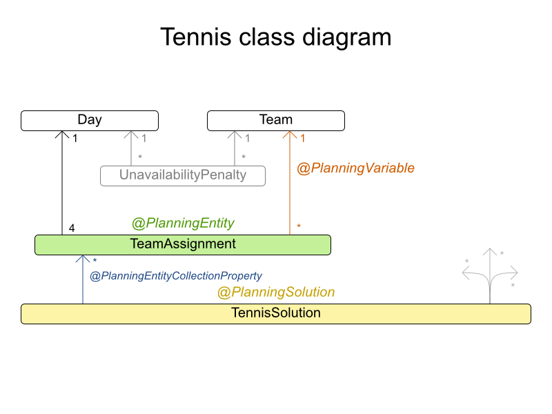
4.8. Meeting scheduling
Assign each meeting to a starting time and a room. Meetings have different durations.
Hard constraints:
- Room conflict: two meetings must not use the same room at the same time.
- Required attendance: A person cannot have two required meetings at the same time.
- Required room capacity: A meeting must not be in a room that doesn’t fit all of the meeting’s attendees.
- Start and end on same day: A meeting shouldn’t be scheduled over multiple days.
Medium constraints:
- Preferred attendance: A person cannot have two preferred meetings at the same time, nor a preferred and a required meeting at the same time.
Soft constraints:
- Sooner rather than later: Schedule all meetings as soon as possible.
- A break between meetings: Any two meetings should have at least one time grain break between them.
- Overlapping meetings: To minimize the number of meetings in parallel so people don’t have to choose one meeting over the other.
- Assign larger rooms first: If a larger room is available any meeting should be assigned to that room in order to accommodate as many people as possible even if they haven’t signed up to that meeting.
- Room stability: If a person has two consecutive meetings with two or less time grains break between them they better be in the same room.
Problem size
50meetings-160timegrains-5rooms  has  50 meetings, 160 timeGrains and 5 rooms with a search space of 10^145.
100meetings-320timegrains-5rooms has 100 meetings, 320 timeGrains and 5 rooms with a search space of 10^320.
200meetings-640timegrains-5rooms has 200 meetings, 640 timeGrains and 5 rooms with a search space of 10^701.
400meetings-1280timegrains-5rooms has 400 meetings, 1280 timeGrains and 5 rooms with a search space of 10^1522.
800meetings-2560timegrains-5rooms has 800 meetings, 2560 timeGrains and 5 rooms with a search space of 10^3285.
4.9. Course timetabling (ITC 2007 Track 3 - Curriculum Course Scheduling)
Schedule each lecture into a timeslot and into a room.
Hard constraints:
- Teacher conflict: A teacher must not have two lectures in the same period.
- Curriculum conflict: A curriculum must not have two lectures in the same period.
- Room occupancy: Two lectures must not be in the same room in the same period.
- Unavailable period (specified per dataset): A specific lecture must not be assigned to a specific period.
Soft constraints:
- Room capacity: A room’s capacity should not be less than the number of students in its lecture.
- Minimum working days: Lectures of the same course should be spread out into a minimum number of days.
- Curriculum compactness: Lectures belonging to the same curriculum should be adjacent to each other (so in consecutive periods).
- Room stability: Lectures of the same course should be assigned to the same room.
The problem is defined by the International Timetabling Competition 2007 track 3.
Problem size
comp01 has 24 teachers,  14 curricula,  30 courses, 160 lectures, 30 periods,  6 rooms and   53 unavailable period constraints with a search space of  10^360.
comp02 has 71 teachers,  70 curricula,  82 courses, 283 lectures, 25 periods, 16 rooms and  513 unavailable period constraints with a search space of  10^736.
comp03 has 61 teachers,  68 curricula,  72 courses, 251 lectures, 25 periods, 16 rooms and  382 unavailable period constraints with a search space of  10^653.
comp04 has 70 teachers,  57 curricula,  79 courses, 286 lectures, 25 periods, 18 rooms and  396 unavailable period constraints with a search space of  10^758.
comp05 has 47 teachers, 139 curricula,  54 courses, 152 lectures, 36 periods,  9 rooms and  771 unavailable period constraints with a search space of  10^381.
comp06 has 87 teachers,  70 curricula, 108 courses, 361 lectures, 25 periods, 18 rooms and  632 unavailable period constraints with a search space of  10^957.
comp07 has 99 teachers,  77 curricula, 131 courses, 434 lectures, 25 periods, 20 rooms and  667 unavailable period constraints with a search space of 10^1171.
comp08 has 76 teachers,  61 curricula,  86 courses, 324 lectures, 25 periods, 18 rooms and  478 unavailable period constraints with a search space of  10^859.
comp09 has 68 teachers,  75 curricula,  76 courses, 279 lectures, 25 periods, 18 rooms and  405 unavailable period constraints with a search space of  10^740.
comp10 has 88 teachers,  67 curricula, 115 courses, 370 lectures, 25 periods, 18 rooms and  694 unavailable period constraints with a search space of  10^981.
comp11 has 24 teachers,  13 curricula,  30 courses, 162 lectures, 45 periods,  5 rooms and   94 unavailable period constraints with a search space of  10^381.
comp12 has 74 teachers, 150 curricula,  88 courses, 218 lectures, 36 periods, 11 rooms and 1368 unavailable period constraints with a search space of  10^566.
comp13 has 77 teachers,  66 curricula,  82 courses, 308 lectures, 25 periods, 19 rooms and  468 unavailable period constraints with a search space of  10^824.
comp14 has 68 teachers,  60 curricula,  85 courses, 275 lectures, 25 periods, 17 rooms and  486 unavailable period constraints with a search space of  10^722.
Figure 4.5. Domain model
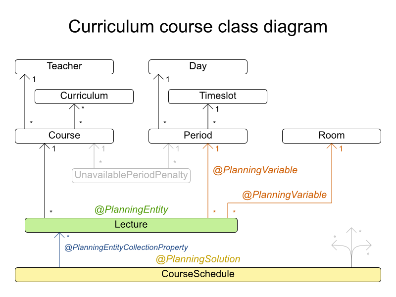
4.10. Machine reassignment (Google ROADEF 2012)
Assign each process to a machine. All processes already have an original (unoptimized) assignment. Each process requires an amount of each resource (such as CPU or RAM). This is a more complex version of the Cloud Balancing example.
Hard constraints:
- Maximum capacity: The maximum capacity for each resource for each machine must not be exceeded.
- Conflict: Processes of the same service must run on distinct machines.
- Spread: Processes of the same service must be spread out across locations.
- Dependency: The processes of a service depending on another service must run in the neighborhood of a process of the other service.
- Transient usage: Some resources are transient and count towards the maximum capacity of both the original machine as the newly assigned machine.
Soft constraints:
- Load: The safety capacity for each resource for each machine should not be exceeded.
- Balance: Leave room for future assignments by balancing the available resources on each machine.
- Process move cost: A process has a move cost.
- Service move cost: A service has a move cost.
- Machine move cost: Moving a process from machine A to machine B has another A-B specific move cost.
The problem is defined by the Google ROADEF/EURO Challenge 2012.
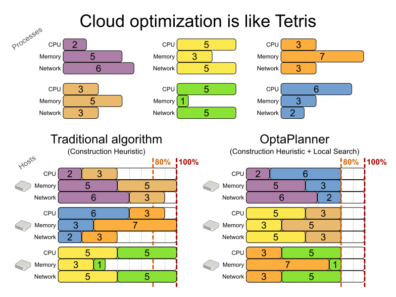
Figure 4.6. Value proposition
Problem size
model_a1_1 has  2 resources,  1 neighborhoods,   4 locations,    4 machines,    79 services,   100 processes and 1 balancePenalties with a search space of     10^60.
model_a1_2 has  4 resources,  2 neighborhoods,   4 locations,  100 machines,   980 services,  1000 processes and 0 balancePenalties with a search space of   10^2000.
model_a1_3 has  3 resources,  5 neighborhoods,  25 locations,  100 machines,   216 services,  1000 processes and 0 balancePenalties with a search space of   10^2000.
model_a1_4 has  3 resources, 50 neighborhoods,  50 locations,   50 machines,   142 services,  1000 processes and 1 balancePenalties with a search space of   10^1698.
model_a1_5 has  4 resources,  2 neighborhoods,   4 locations,   12 machines,   981 services,  1000 processes and 1 balancePenalties with a search space of   10^1079.
model_a2_1 has  3 resources,  1 neighborhoods,   1 locations,  100 machines,  1000 services,  1000 processes and 0 balancePenalties with a search space of   10^2000.
model_a2_2 has 12 resources,  5 neighborhoods,  25 locations,  100 machines,   170 services,  1000 processes and 0 balancePenalties with a search space of   10^2000.
model_a2_3 has 12 resources,  5 neighborhoods,  25 locations,  100 machines,   129 services,  1000 processes and 0 balancePenalties with a search space of   10^2000.
model_a2_4 has 12 resources,  5 neighborhoods,  25 locations,   50 machines,   180 services,  1000 processes and 1 balancePenalties with a search space of   10^1698.
model_a2_5 has 12 resources,  5 neighborhoods,  25 locations,   50 machines,   153 services,  1000 processes and 0 balancePenalties with a search space of   10^1698.
model_b_1  has 12 resources,  5 neighborhoods,  10 locations,  100 machines,  2512 services,  5000 processes and 0 balancePenalties with a search space of  10^10000.
model_b_2  has 12 resources,  5 neighborhoods,  10 locations,  100 machines,  2462 services,  5000 processes and 1 balancePenalties with a search space of  10^10000.
model_b_3  has  6 resources,  5 neighborhoods,  10 locations,  100 machines, 15025 services, 20000 processes and 0 balancePenalties with a search space of  10^40000.
model_b_4  has  6 resources,  5 neighborhoods,  50 locations,  500 machines,  1732 services, 20000 processes and 1 balancePenalties with a search space of  10^53979.
model_b_5  has  6 resources,  5 neighborhoods,  10 locations,  100 machines, 35082 services, 40000 processes and 0 balancePenalties with a search space of  10^80000.
model_b_6  has  6 resources,  5 neighborhoods,  50 locations,  200 machines, 14680 services, 40000 processes and 1 balancePenalties with a search space of  10^92041.
model_b_7  has  6 resources,  5 neighborhoods,  50 locations, 4000 machines, 15050 services, 40000 processes and 1 balancePenalties with a search space of 10^144082.
model_b_8  has  3 resources,  5 neighborhoods,  10 locations,  100 machines, 45030 services, 50000 processes and 0 balancePenalties with a search space of 10^100000.
model_b_9  has  3 resources,  5 neighborhoods, 100 locations, 1000 machines,  4609 services, 50000 processes and 1 balancePenalties with a search space of 10^150000.
model_b_10 has  3 resources,  5 neighborhoods, 100 locations, 5000 machines,  4896 services, 50000 processes and 1 balancePenalties with a search space of 10^184948.
Figure 4.7. Domain model

4.11. Vehicle routing
Using a fleet of vehicles, pick up the objects of each customer and bring them to the depot. Each vehicle can service multiple customers, but it has a limited capacity.
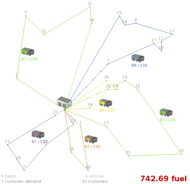
Besides the basic case (CVRP), there is also a variant with time windows (CVRPTW).
Hard constraints:
- Vehicle capacity: a vehicle cannot carry more items then its capacity.
Time windows (only in CVRPTW):
- Travel time: Traveling from one location to another takes time.
- Customer service duration: a vehicle must stay at the customer for the length of the service duration.
- Customer ready time: a vehicle may arrive before the customer’s ready time, but it must wait until the ready time before servicing.
- Customer due time: a vehicle must arrive on time, before the customer’s due time.
Soft constraints:
- Total distance: minimize the total distance driven (fuel consumption) of all vehicles.
The capacitated vehicle routing problem (CVRP) and its timewindowed variant (CVRPTW) are defined by the VRP web.
Figure 4.8. Value proposition

Problem size
CVRP instances (without time windows):
belgium-n50-k10             has  1 depots, 10 vehicles and   49 customers with a search space of   10^74.
belgium-n100-k10            has  1 depots, 10 vehicles and   99 customers with a search space of  10^170.
belgium-n500-k20            has  1 depots, 20 vehicles and  499 customers with a search space of 10^1168.
belgium-n1000-k20           has  1 depots, 20 vehicles and  999 customers with a search space of 10^2607.
belgium-n2750-k55           has  1 depots, 55 vehicles and 2749 customers with a search space of 10^8380.
belgium-road-km-n50-k10     has  1 depots, 10 vehicles and   49 customers with a search space of   10^74.
belgium-road-km-n100-k10    has  1 depots, 10 vehicles and   99 customers with a search space of  10^170.
belgium-road-km-n500-k20    has  1 depots, 20 vehicles and  499 customers with a search space of 10^1168.
belgium-road-km-n1000-k20   has  1 depots, 20 vehicles and  999 customers with a search space of 10^2607.
belgium-road-km-n2750-k55   has  1 depots, 55 vehicles and 2749 customers with a search space of 10^8380.
belgium-road-time-n50-k10   has  1 depots, 10 vehicles and   49 customers with a search space of   10^74.
belgium-road-time-n100-k10  has  1 depots, 10 vehicles and   99 customers with a search space of  10^170.
belgium-road-time-n500-k20  has  1 depots, 20 vehicles and  499 customers with a search space of 10^1168.
belgium-road-time-n1000-k20 has  1 depots, 20 vehicles and  999 customers with a search space of 10^2607.
belgium-road-time-n2750-k55 has  1 depots, 55 vehicles and 2749 customers with a search space of 10^8380.
belgium-d2-n50-k10          has  2 depots, 10 vehicles and   48 customers with a search space of   10^74.
belgium-d3-n100-k10         has  3 depots, 10 vehicles and   97 customers with a search space of  10^170.
belgium-d5-n500-k20         has  5 depots, 20 vehicles and  495 customers with a search space of 10^1168.
belgium-d8-n1000-k20        has  8 depots, 20 vehicles and  992 customers with a search space of 10^2607.
belgium-d10-n2750-k55       has 10 depots, 55 vehicles and 2740 customers with a search space of 10^8380.

A-n32-k5  has 1 depots,  5 vehicles and  31 customers with a search space of  10^40.
A-n33-k5  has 1 depots,  5 vehicles and  32 customers with a search space of  10^41.
A-n33-k6  has 1 depots,  6 vehicles and  32 customers with a search space of  10^42.
A-n34-k5  has 1 depots,  5 vehicles and  33 customers with a search space of  10^43.
A-n36-k5  has 1 depots,  5 vehicles and  35 customers with a search space of  10^46.
A-n37-k5  has 1 depots,  5 vehicles and  36 customers with a search space of  10^48.
A-n37-k6  has 1 depots,  6 vehicles and  36 customers with a search space of  10^49.
A-n38-k5  has 1 depots,  5 vehicles and  37 customers with a search space of  10^49.
A-n39-k5  has 1 depots,  5 vehicles and  38 customers with a search space of  10^51.
A-n39-k6  has 1 depots,  6 vehicles and  38 customers with a search space of  10^52.
A-n44-k7  has 1 depots,  7 vehicles and  43 customers with a search space of  10^61.
A-n45-k6  has 1 depots,  6 vehicles and  44 customers with a search space of  10^62.
A-n45-k7  has 1 depots,  7 vehicles and  44 customers with a search space of  10^63.
A-n46-k7  has 1 depots,  7 vehicles and  45 customers with a search space of  10^65.
A-n48-k7  has 1 depots,  7 vehicles and  47 customers with a search space of  10^68.
A-n53-k7  has 1 depots,  7 vehicles and  52 customers with a search space of  10^77.
A-n54-k7  has 1 depots,  7 vehicles and  53 customers with a search space of  10^79.
A-n55-k9  has 1 depots,  9 vehicles and  54 customers with a search space of  10^82.
A-n60-k9  has 1 depots,  9 vehicles and  59 customers with a search space of  10^91.
A-n61-k9  has 1 depots,  9 vehicles and  60 customers with a search space of  10^93.
A-n62-k8  has 1 depots,  8 vehicles and  61 customers with a search space of  10^94.
A-n63-k9  has 1 depots,  9 vehicles and  62 customers with a search space of  10^97.
A-n63-k10 has 1 depots, 10 vehicles and  62 customers with a search space of  10^98.
A-n64-k9  has 1 depots,  9 vehicles and  63 customers with a search space of  10^99.
A-n65-k9  has 1 depots,  9 vehicles and  64 customers with a search space of 10^101.
A-n69-k9  has 1 depots,  9 vehicles and  68 customers with a search space of 10^108.
A-n80-k10 has 1 depots, 10 vehicles and  79 customers with a search space of 10^130.
F-n45-k4  has 1 depots,  4 vehicles and  44 customers with a search space of  10^60.
F-n72-k4  has 1 depots,  4 vehicles and  71 customers with a search space of 10^108.
F-n135-k7 has 1 depots,  7 vehicles and 134 customers with a search space of 10^240.
CVRPTW instances (with time windows):
belgium-tw-d2-n50-k10    has  2 depots, 10 vehicles and   48 customers with a search space of   10^74.
belgium-tw-d3-n100-k10   has  3 depots, 10 vehicles and   97 customers with a search space of  10^170.
belgium-tw-d5-n500-k20   has  5 depots, 20 vehicles and  495 customers with a search space of 10^1168.
belgium-tw-d8-n1000-k20  has  8 depots, 20 vehicles and  992 customers with a search space of 10^2607.
belgium-tw-d10-n2750-k55 has 10 depots, 55 vehicles and 2740 customers with a search space of 10^8380.
belgium-tw-n50-k10       has  1 depots, 10 vehicles and   49 customers with a search space of   10^74.
belgium-tw-n100-k10      has  1 depots, 10 vehicles and   99 customers with a search space of  10^170.
belgium-tw-n500-k20      has  1 depots, 20 vehicles and  499 customers with a search space of 10^1168.
belgium-tw-n1000-k20     has  1 depots, 20 vehicles and  999 customers with a search space of 10^2607.
belgium-tw-n2750-k55     has  1 depots, 55 vehicles and 2749 customers with a search space of 10^8380.

Solomon_025_C101       has 1 depots,  25 vehicles and   25 customers with a search space of   10^40.
Solomon_025_C201       has 1 depots,  25 vehicles and   25 customers with a search space of   10^40.
Solomon_025_R101       has 1 depots,  25 vehicles and   25 customers with a search space of   10^40.
Solomon_025_R201       has 1 depots,  25 vehicles and   25 customers with a search space of   10^40.
Solomon_025_RC101      has 1 depots,  25 vehicles and   25 customers with a search space of   10^40.
Solomon_025_RC201      has 1 depots,  25 vehicles and   25 customers with a search space of   10^40.
Solomon_100_C101       has 1 depots,  25 vehicles and  100 customers with a search space of  10^185.
Solomon_100_C201       has 1 depots,  25 vehicles and  100 customers with a search space of  10^185.
Solomon_100_R101       has 1 depots,  25 vehicles and  100 customers with a search space of  10^185.
Solomon_100_R201       has 1 depots,  25 vehicles and  100 customers with a search space of  10^185.
Solomon_100_RC101      has 1 depots,  25 vehicles and  100 customers with a search space of  10^185.
Solomon_100_RC201      has 1 depots,  25 vehicles and  100 customers with a search space of  10^185.
Homberger_0200_C1_2_1  has 1 depots,  50 vehicles and  200 customers with a search space of  10^429.
Homberger_0200_C2_2_1  has 1 depots,  50 vehicles and  200 customers with a search space of  10^429.
Homberger_0200_R1_2_1  has 1 depots,  50 vehicles and  200 customers with a search space of  10^429.
Homberger_0200_R2_2_1  has 1 depots,  50 vehicles and  200 customers with a search space of  10^429.
Homberger_0200_RC1_2_1 has 1 depots,  50 vehicles and  200 customers with a search space of  10^429.
Homberger_0200_RC2_2_1 has 1 depots,  50 vehicles and  200 customers with a search space of  10^429.
Homberger_0400_C1_4_1  has 1 depots, 100 vehicles and  400 customers with a search space of  10^978.
Homberger_0400_C2_4_1  has 1 depots, 100 vehicles and  400 customers with a search space of  10^978.
Homberger_0400_R1_4_1  has 1 depots, 100 vehicles and  400 customers with a search space of  10^978.
Homberger_0400_R2_4_1  has 1 depots, 100 vehicles and  400 customers with a search space of  10^978.
Homberger_0400_RC1_4_1 has 1 depots, 100 vehicles and  400 customers with a search space of  10^978.
Homberger_0400_RC2_4_1 has 1 depots, 100 vehicles and  400 customers with a search space of  10^978.
Homberger_0600_C1_6_1  has 1 depots, 150 vehicles and  600 customers with a search space of 10^1571.
Homberger_0600_C2_6_1  has 1 depots, 150 vehicles and  600 customers with a search space of 10^1571.
Homberger_0600_R1_6_1  has 1 depots, 150 vehicles and  600 customers with a search space of 10^1571.
Homberger_0600_R2_6_1  has 1 depots, 150 vehicles and  600 customers with a search space of 10^1571.
Homberger_0600_RC1_6_1 has 1 depots, 150 vehicles and  600 customers with a search space of 10^1571.
Homberger_0600_RC2_6_1 has 1 depots, 150 vehicles and  600 customers with a search space of 10^1571.
Homberger_0800_C1_8_1  has 1 depots, 200 vehicles and  800 customers with a search space of 10^2195.
Homberger_0800_C2_8_1  has 1 depots, 200 vehicles and  800 customers with a search space of 10^2195.
Homberger_0800_R1_8_1  has 1 depots, 200 vehicles and  800 customers with a search space of 10^2195.
Homberger_0800_R2_8_1  has 1 depots, 200 vehicles and  800 customers with a search space of 10^2195.
Homberger_0800_RC1_8_1 has 1 depots, 200 vehicles and  800 customers with a search space of 10^2195.
Homberger_0800_RC2_8_1 has 1 depots, 200 vehicles and  800 customers with a search space of 10^2195.
Homberger_1000_C110_1  has 1 depots, 250 vehicles and 1000 customers with a search space of 10^2840.
Homberger_1000_C210_1  has 1 depots, 250 vehicles and 1000 customers with a search space of 10^2840.
Homberger_1000_R110_1  has 1 depots, 250 vehicles and 1000 customers with a search space of 10^2840.
Homberger_1000_R210_1  has 1 depots, 250 vehicles and 1000 customers with a search space of 10^2840.
Homberger_1000_RC110_1 has 1 depots, 250 vehicles and 1000 customers with a search space of 10^2840.
Homberger_1000_RC210_1 has 1 depots, 250 vehicles and 1000 customers with a search space of 10^2840.
4.11.1. Domain model for Vehicle routing
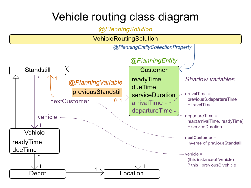
The vehicle routing with timewindows domain model makes heavily use of the shadow variable feature. This allows it to express its constraints more naturally, because properties such as arrivalTime and departureTime, are directly available on the domain model.
Road Distances Instead of Air Distances
In the real world, vehicles cannot follow a straight line from location to location: they have to use roads and highways. From a business point of view, this matters a lot:
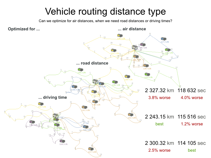
For the optimization algorithm, this does not matter much, as long as the distance between two points can be looked up (and are preferably precalculated). The road cost does not even need to be a distance, it can also be travel time, fuel cost, or a weighted function of those. There are several technologies available to precalculate road costs, such as GraphHopper (embeddable, offline Java engine), Open MapQuest (web service) and Google Maps Client API (web service).
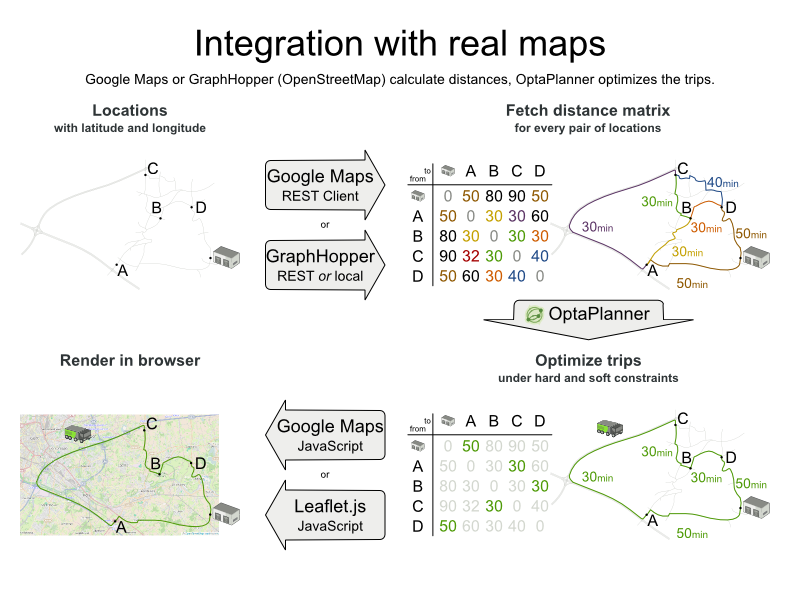
There are also several technologies to render it, such as Leaflet and Google Maps for developers: the optaplanner-webexamples-*.war has an example which demonstrates such rendering:

It is even possible to render the actual road routes with GraphHopper or Google Map Directions, but because of route overlaps on highways, it can become harder to see the standstill order:
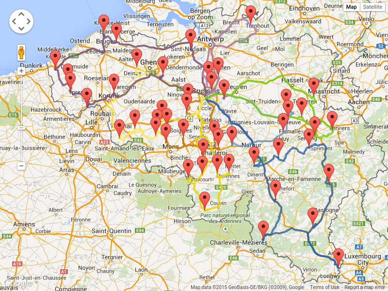
Take special care that the road costs between two points use the same optimization criteria as the one used in Planner. For example, GraphHopper etc will by default return the fastest route, not the shortest route. Don’t use the km (or miles) distances of the fastest GPS routes to optimize the shortest trip in Planner: this leads to a suboptimal solution as shown below:
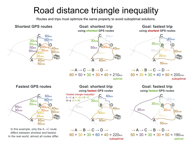
Contrary to popular belief, most users do not want the shortest route: they want the fastest route instead. They prefer highways over normal roads. They prefer normal roads over dirt roads. In the real world, the fastest and shortest route are rarely the same.
4.12. Project job scheduling
Schedule all jobs in time and execution mode to minimize project delays. Each job is part of a project. A job can be executed in different ways: each way is an execution mode that implies a different duration but also different resource usages. This is a form of flexible job shop scheduling.
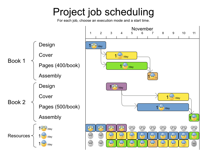
Hard constraints:
- Job precedence: a job can only start when all its predecessor jobs are finished.
Resource capacity: do not use more resources than available.
- Resources are local (shared between jobs of the same project) or global (shared between all jobs)
- Resources are renewable (capacity available per day) or nonrenewable (capacity available for all days)
Medium constraints:
- Total project delay: minimize the duration (makespan) of each project.
Soft constraints:
- Total makespan: minimize the duration of the whole multi-project schedule.
The problem is defined by the MISTA 2013 challenge.
Problem size
Schedule A-1  has  2 projects,  24 jobs,   64 execution modes,  7 resources and  150 resource requirements.
Schedule A-2  has  2 projects,  44 jobs,  124 execution modes,  7 resources and  420 resource requirements.
Schedule A-3  has  2 projects,  64 jobs,  184 execution modes,  7 resources and  630 resource requirements.
Schedule A-4  has  5 projects,  60 jobs,  160 execution modes, 16 resources and  390 resource requirements.
Schedule A-5  has  5 projects, 110 jobs,  310 execution modes, 16 resources and  900 resource requirements.
Schedule A-6  has  5 projects, 160 jobs,  460 execution modes, 16 resources and 1440 resource requirements.
Schedule A-7  has 10 projects, 120 jobs,  320 execution modes, 22 resources and  900 resource requirements.
Schedule A-8  has 10 projects, 220 jobs,  620 execution modes, 22 resources and 1860 resource requirements.
Schedule A-9  has 10 projects, 320 jobs,  920 execution modes, 31 resources and 2880 resource requirements.
Schedule A-10 has 10 projects, 320 jobs,  920 execution modes, 31 resources and 2970 resource requirements.
Schedule B-1  has 10 projects, 120 jobs,  320 execution modes, 31 resources and  900 resource requirements.
Schedule B-2  has 10 projects, 220 jobs,  620 execution modes, 22 resources and 1740 resource requirements.
Schedule B-3  has 10 projects, 320 jobs,  920 execution modes, 31 resources and 3060 resource requirements.
Schedule B-4  has 15 projects, 180 jobs,  480 execution modes, 46 resources and 1530 resource requirements.
Schedule B-5  has 15 projects, 330 jobs,  930 execution modes, 46 resources and 2760 resource requirements.
Schedule B-6  has 15 projects, 480 jobs, 1380 execution modes, 46 resources and 4500 resource requirements.
Schedule B-7  has 20 projects, 240 jobs,  640 execution modes, 61 resources and 1710 resource requirements.
Schedule B-8  has 20 projects, 440 jobs, 1240 execution modes, 42 resources and 3180 resource requirements.
Schedule B-9  has 20 projects, 640 jobs, 1840 execution modes, 61 resources and 5940 resource requirements.
Schedule B-10 has 20 projects, 460 jobs, 1300 execution modes, 42 resources and 4260 resource requirements.
4.13. Task assigning
Assign each task to a spot in an employee’s queue. Each task has a duration which is affected by the employee’s affinity level with the task’s customer.
Hard constraints:
- Skill: Each task requires one or more skills. The employee must possess all these skills.
Soft level 0 constraints:
- Critical tasks: Complete critical tasks first, sooner than major and minor tasks.
Soft level 1 constraints:
Minimize makespan: Reduce the time to complete all tasks.
- Start with the longest working employee first, then the second longest working employee and so forth, to create fairness and load balancing.
Soft level 2 constraints:
- Major tasks: Complete major tasks as soon as possible, sooner than minor tasks.
Soft level 3 constraints:
- Minor tasks: Complete minor tasks as soon as possible.
Figure 4.9. Value proposition
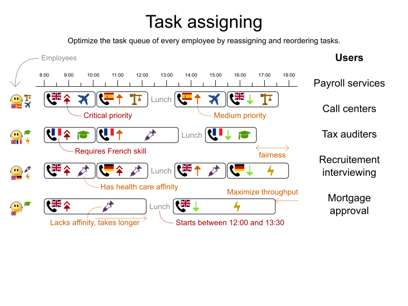
Problem size
24tasks-8employees   has  24 tasks, 6 skills,  8 employees,   4 task types and  4 customers with a search space of   10^30.
50tasks-5employees   has  50 tasks, 5 skills,  5 employees,  10 task types and 10 customers with a search space of   10^69.
100tasks-5employees  has 100 tasks, 5 skills,  5 employees,  20 task types and 15 customers with a search space of  10^164.
500tasks-20employees has 500 tasks, 6 skills, 20 employees, 100 task types and 60 customers with a search space of 10^1168.
Figure 4.10. Domain model

4.14. Exam timetabling (ITC 2007 track 1 - Examination)
Schedule each exam into a period and into a room. Multiple exams can share the same room during the same period.
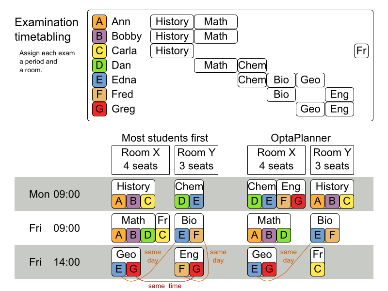
Hard constraints:
- Exam conflict: Two exams that share students must not occur in the same period.
- Room capacity: A room’s seating capacity must suffice at all times.
- Period duration: A period’s duration must suffice for all of its exams.
Period related hard constraints (specified per dataset):
- Coincidence: Two specified exams must use the same period (but possibly another room).
- Exclusion: Two specified exams must not use the same period.
- After: A specified exam must occur in a period after another specified exam’s period.
Room related hard constraints (specified per dataset):
- Exclusive: One specified exam should not have to share its room with any other exam.
Soft constraints (each of which has a parametrized penalty):
- The same student should not have two exams in a row.
- The same student should not have two exams on the same day.
- Period spread: Two exams that share students should be a number of periods apart.
- Mixed durations: Two exams that share a room should not have different durations.
- Front load: Large exams should be scheduled earlier in the schedule.
- Period penalty (specified per dataset): Some periods have a penalty when used.
- Room penalty (specified per dataset): Some rooms have a penalty when used.
It uses large test data sets of real-life universities.
The problem is defined by the International Timetabling Competition 2007 track 1. Geoffrey De Smet finished 4th in that competition with a very early version of Planner. Many improvements have been made since then.
Problem Size
exam_comp_set1 has  7883 students,  607 exams, 54 periods,  7 rooms,  12 period constraints and  0 room constraints with a search space of 10^1564.
exam_comp_set2 has 12484 students,  870 exams, 40 periods, 49 rooms,  12 period constraints and  2 room constraints with a search space of 10^2864.
exam_comp_set3 has 16365 students,  934 exams, 36 periods, 48 rooms, 168 period constraints and 15 room constraints with a search space of 10^3023.
exam_comp_set4 has  4421 students,  273 exams, 21 periods,  1 rooms,  40 period constraints and  0 room constraints with a search space of  10^360.
exam_comp_set5 has  8719 students, 1018 exams, 42 periods,  3 rooms,  27 period constraints and  0 room constraints with a search space of 10^2138.
exam_comp_set6 has  7909 students,  242 exams, 16 periods,  8 rooms,  22 period constraints and  0 room constraints with a search space of  10^509.
exam_comp_set7 has 13795 students, 1096 exams, 80 periods, 15 rooms,  28 period constraints and  0 room constraints with a search space of 10^3374.
exam_comp_set8 has  7718 students,  598 exams, 80 periods,  8 rooms,  20 period constraints and  1 room constraints with a search space of 10^1678.
4.14.1. Domain model for Exam timetabling
The following diagram shows the main examination domain classes:
Figure 4.11. Examination domain class diagram
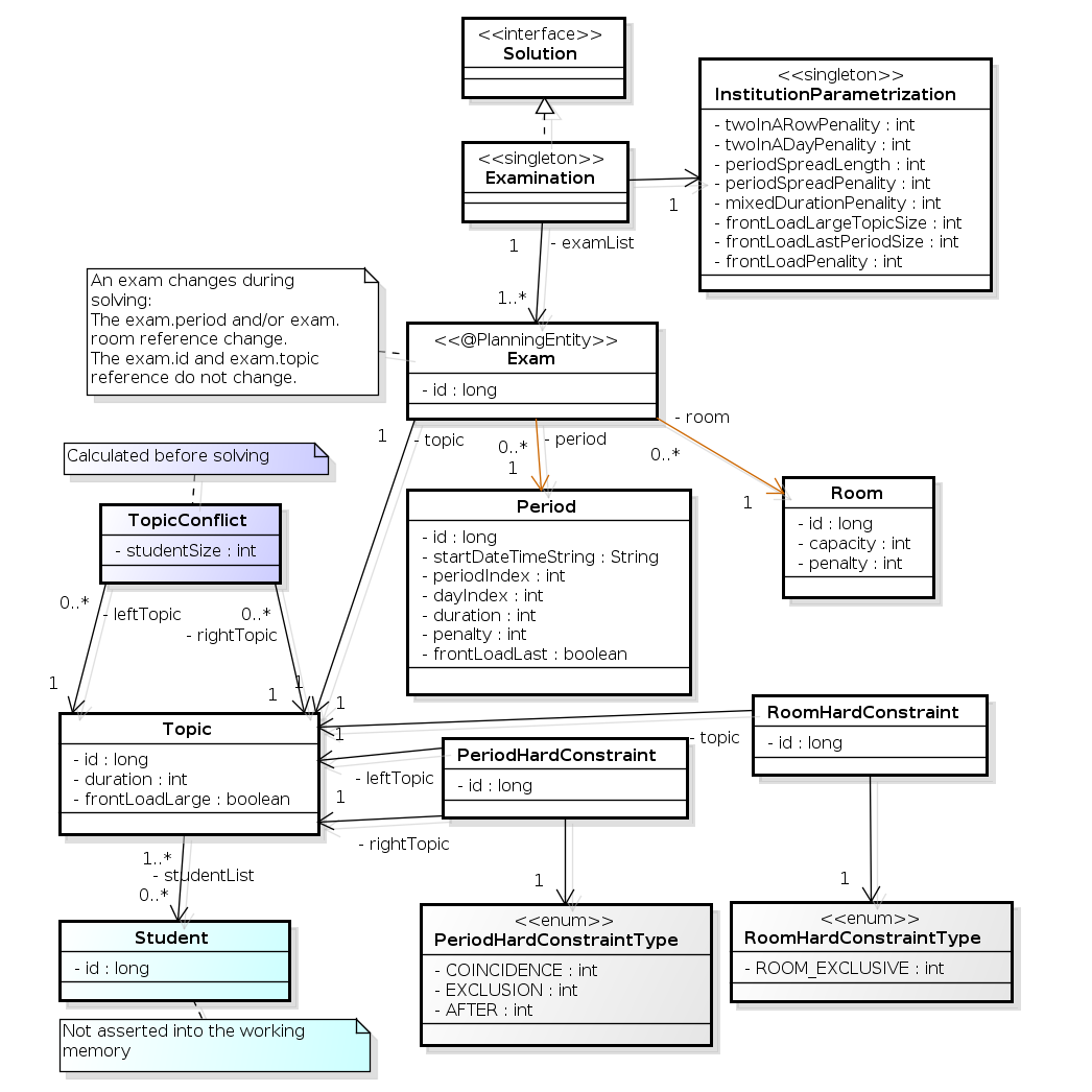
Notice that we’ve split up the exam concept into an Exam class and a Topic class. The Exam instances change during solving (this is the planning entity class), when their period or room property changes. The Topic, Period and Room instances never change during solving (these are problem facts, just like some other classes).
4.15. Nurse rostering (INRC 2010)
For each shift, assign a nurse to work that shift.
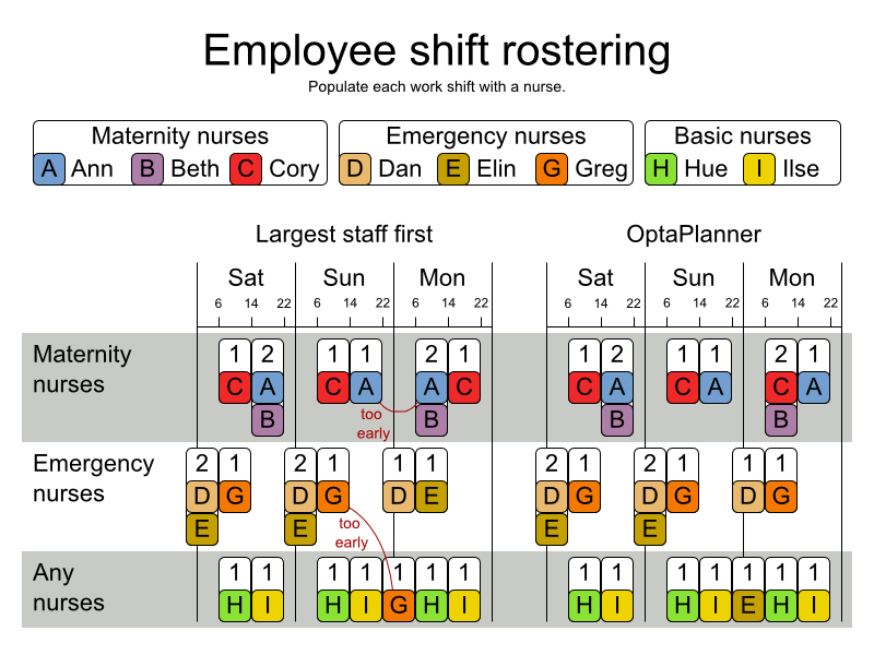
Hard constraints:
- No unassigned shifts (built-in): Every shift need to be assigned to an employee.
- Shift conflict: An employee can have only one shift per day.
Soft constraints:
Contract obligations. The business frequently violates these, so they decided to define these as soft constraints instead of hard constraints.
- Minimum and maximum assignments: Each employee needs to work more than x shifts and less than y shifts (depending on their contract).
- Minimum and maximum consecutive working days: Each employee needs to work between x and y days in a row (depending on their contract).
- Minimum and maximum consecutive free days: Each employee needs to be free between x and y days in a row (depending on their contract).
- Minimum and maximum consecutive working weekends: Each employee needs to work between x and y weekends in a row (depending on their contract).
- Complete weekends: Each employee needs to work every day in a weekend or not at all.
- Identical shift types during weekend: Each weekend shift for the same weekend of the same employee must be the same shift type.
- Unwanted patterns: A combination of unwanted shift types in a row. For example: a late shift followed by an early shift followed by a late shift.
Employee wishes:
- Day on request: An employee wants to work on a specific day.
- Day off request: An employee does not want to work on a specific day.
- Shift on request: An employee wants to be assigned to a specific shift.
- Shift off request: An employee does not want to be assigned to a specific shift.
- Alternative skill: An employee assigned to a skill should have a proficiency in every skill required by that shift.
The problem is defined by the International Nurse Rostering Competition 2010.
Figure 4.12. Value proposition
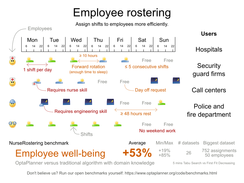
Problem size
There are three dataset types:
- sprint: must be solved in seconds.
- medium: must be solved in minutes.
- long: must be solved in hours.
toy1          has 1 skills, 3 shiftTypes, 2 patterns, 1 contracts,  6 employees,  7 shiftDates,  35 shiftAssignments and   0 requests with a search space of   10^27.
toy2          has 1 skills, 3 shiftTypes, 3 patterns, 2 contracts, 20 employees, 28 shiftDates, 180 shiftAssignments and 140 requests with a search space of  10^234.

sprint01      has 1 skills, 4 shiftTypes, 3 patterns, 4 contracts, 10 employees, 28 shiftDates, 152 shiftAssignments and 150 requests with a search space of  10^152.
sprint02      has 1 skills, 4 shiftTypes, 3 patterns, 4 contracts, 10 employees, 28 shiftDates, 152 shiftAssignments and 150 requests with a search space of  10^152.
sprint03      has 1 skills, 4 shiftTypes, 3 patterns, 4 contracts, 10 employees, 28 shiftDates, 152 shiftAssignments and 150 requests with a search space of  10^152.
sprint04      has 1 skills, 4 shiftTypes, 3 patterns, 4 contracts, 10 employees, 28 shiftDates, 152 shiftAssignments and 150 requests with a search space of  10^152.
sprint05      has 1 skills, 4 shiftTypes, 3 patterns, 4 contracts, 10 employees, 28 shiftDates, 152 shiftAssignments and 150 requests with a search space of  10^152.
sprint06      has 1 skills, 4 shiftTypes, 3 patterns, 4 contracts, 10 employees, 28 shiftDates, 152 shiftAssignments and 150 requests with a search space of  10^152.
sprint07      has 1 skills, 4 shiftTypes, 3 patterns, 4 contracts, 10 employees, 28 shiftDates, 152 shiftAssignments and 150 requests with a search space of  10^152.
sprint08      has 1 skills, 4 shiftTypes, 3 patterns, 4 contracts, 10 employees, 28 shiftDates, 152 shiftAssignments and 150 requests with a search space of  10^152.
sprint09      has 1 skills, 4 shiftTypes, 3 patterns, 4 contracts, 10 employees, 28 shiftDates, 152 shiftAssignments and 150 requests with a search space of  10^152.
sprint10      has 1 skills, 4 shiftTypes, 3 patterns, 4 contracts, 10 employees, 28 shiftDates, 152 shiftAssignments and 150 requests with a search space of  10^152.
sprint_hint01 has 1 skills, 4 shiftTypes, 8 patterns, 3 contracts, 10 employees, 28 shiftDates, 152 shiftAssignments and 150 requests with a search space of  10^152.
sprint_hint02 has 1 skills, 4 shiftTypes, 0 patterns, 3 contracts, 10 employees, 28 shiftDates, 152 shiftAssignments and 150 requests with a search space of  10^152.
sprint_hint03 has 1 skills, 4 shiftTypes, 8 patterns, 3 contracts, 10 employees, 28 shiftDates, 152 shiftAssignments and 150 requests with a search space of  10^152.
sprint_late01 has 1 skills, 4 shiftTypes, 8 patterns, 3 contracts, 10 employees, 28 shiftDates, 152 shiftAssignments and 150 requests with a search space of  10^152.
sprint_late02 has 1 skills, 3 shiftTypes, 4 patterns, 3 contracts, 10 employees, 28 shiftDates, 144 shiftAssignments and 139 requests with a search space of  10^144.
sprint_late03 has 1 skills, 4 shiftTypes, 8 patterns, 3 contracts, 10 employees, 28 shiftDates, 160 shiftAssignments and 150 requests with a search space of  10^160.
sprint_late04 has 1 skills, 4 shiftTypes, 8 patterns, 3 contracts, 10 employees, 28 shiftDates, 160 shiftAssignments and 150 requests with a search space of  10^160.
sprint_late05 has 1 skills, 4 shiftTypes, 8 patterns, 3 contracts, 10 employees, 28 shiftDates, 152 shiftAssignments and 150 requests with a search space of  10^152.
sprint_late06 has 1 skills, 4 shiftTypes, 0 patterns, 3 contracts, 10 employees, 28 shiftDates, 152 shiftAssignments and 150 requests with a search space of  10^152.
sprint_late07 has 1 skills, 4 shiftTypes, 0 patterns, 3 contracts, 10 employees, 28 shiftDates, 152 shiftAssignments and 150 requests with a search space of  10^152.
sprint_late08 has 1 skills, 4 shiftTypes, 0 patterns, 3 contracts, 10 employees, 28 shiftDates, 152 shiftAssignments and   0 requests with a search space of  10^152.
sprint_late09 has 1 skills, 4 shiftTypes, 0 patterns, 3 contracts, 10 employees, 28 shiftDates, 152 shiftAssignments and   0 requests with a search space of  10^152.
sprint_late10 has 1 skills, 4 shiftTypes, 0 patterns, 3 contracts, 10 employees, 28 shiftDates, 152 shiftAssignments and 150 requests with a search space of  10^152.

medium01      has 1 skills, 4 shiftTypes, 0 patterns, 4 contracts, 31 employees, 28 shiftDates, 608 shiftAssignments and 403 requests with a search space of  10^906.
medium02      has 1 skills, 4 shiftTypes, 0 patterns, 4 contracts, 31 employees, 28 shiftDates, 608 shiftAssignments and 403 requests with a search space of  10^906.
medium03      has 1 skills, 4 shiftTypes, 0 patterns, 4 contracts, 31 employees, 28 shiftDates, 608 shiftAssignments and 403 requests with a search space of  10^906.
medium04      has 1 skills, 4 shiftTypes, 0 patterns, 4 contracts, 31 employees, 28 shiftDates, 608 shiftAssignments and 403 requests with a search space of  10^906.
medium05      has 1 skills, 4 shiftTypes, 0 patterns, 4 contracts, 31 employees, 28 shiftDates, 608 shiftAssignments and 403 requests with a search space of  10^906.
medium_hint01 has 1 skills, 4 shiftTypes, 7 patterns, 4 contracts, 30 employees, 28 shiftDates, 428 shiftAssignments and 390 requests with a search space of  10^632.
medium_hint02 has 1 skills, 4 shiftTypes, 7 patterns, 3 contracts, 30 employees, 28 shiftDates, 428 shiftAssignments and 390 requests with a search space of  10^632.
medium_hint03 has 1 skills, 4 shiftTypes, 7 patterns, 4 contracts, 30 employees, 28 shiftDates, 428 shiftAssignments and 390 requests with a search space of  10^632.
medium_late01 has 1 skills, 4 shiftTypes, 7 patterns, 4 contracts, 30 employees, 28 shiftDates, 424 shiftAssignments and 390 requests with a search space of  10^626.
medium_late02 has 1 skills, 4 shiftTypes, 7 patterns, 3 contracts, 30 employees, 28 shiftDates, 428 shiftAssignments and 390 requests with a search space of  10^632.
medium_late03 has 1 skills, 4 shiftTypes, 0 patterns, 4 contracts, 30 employees, 28 shiftDates, 428 shiftAssignments and 390 requests with a search space of  10^632.
medium_late04 has 1 skills, 4 shiftTypes, 7 patterns, 3 contracts, 30 employees, 28 shiftDates, 416 shiftAssignments and 390 requests with a search space of  10^614.
medium_late05 has 2 skills, 5 shiftTypes, 7 patterns, 4 contracts, 30 employees, 28 shiftDates, 452 shiftAssignments and 390 requests with a search space of  10^667.

long01        has 2 skills, 5 shiftTypes, 3 patterns, 3 contracts, 49 employees, 28 shiftDates, 740 shiftAssignments and 735 requests with a search space of 10^1250.
long02        has 2 skills, 5 shiftTypes, 3 patterns, 3 contracts, 49 employees, 28 shiftDates, 740 shiftAssignments and 735 requests with a search space of 10^1250.
long03        has 2 skills, 5 shiftTypes, 3 patterns, 3 contracts, 49 employees, 28 shiftDates, 740 shiftAssignments and 735 requests with a search space of 10^1250.
long04        has 2 skills, 5 shiftTypes, 3 patterns, 3 contracts, 49 employees, 28 shiftDates, 740 shiftAssignments and 735 requests with a search space of 10^1250.
long05        has 2 skills, 5 shiftTypes, 3 patterns, 3 contracts, 49 employees, 28 shiftDates, 740 shiftAssignments and 735 requests with a search space of 10^1250.
long_hint01   has 2 skills, 5 shiftTypes, 9 patterns, 3 contracts, 50 employees, 28 shiftDates, 740 shiftAssignments and   0 requests with a search space of 10^1257.
long_hint02   has 2 skills, 5 shiftTypes, 7 patterns, 3 contracts, 50 employees, 28 shiftDates, 740 shiftAssignments and   0 requests with a search space of 10^1257.
long_hint03   has 2 skills, 5 shiftTypes, 7 patterns, 3 contracts, 50 employees, 28 shiftDates, 740 shiftAssignments and   0 requests with a search space of 10^1257.
long_late01   has 2 skills, 5 shiftTypes, 9 patterns, 3 contracts, 50 employees, 28 shiftDates, 752 shiftAssignments and   0 requests with a search space of 10^1277.
long_late02   has 2 skills, 5 shiftTypes, 9 patterns, 4 contracts, 50 employees, 28 shiftDates, 752 shiftAssignments and   0 requests with a search space of 10^1277.
long_late03   has 2 skills, 5 shiftTypes, 9 patterns, 3 contracts, 50 employees, 28 shiftDates, 752 shiftAssignments and   0 requests with a search space of 10^1277.
long_late04   has 2 skills, 5 shiftTypes, 9 patterns, 4 contracts, 50 employees, 28 shiftDates, 752 shiftAssignments and   0 requests with a search space of 10^1277.
long_late05   has 2 skills, 5 shiftTypes, 9 patterns, 3 contracts, 50 employees, 28 shiftDates, 740 shiftAssignments and   0 requests with a search space of 10^1257.
Figure 4.13. Domain model
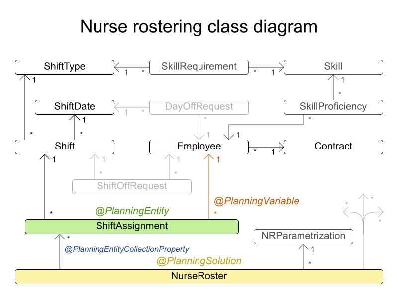
4.16. Traveling tournament problem (TTP)
Schedule matches between n teams.
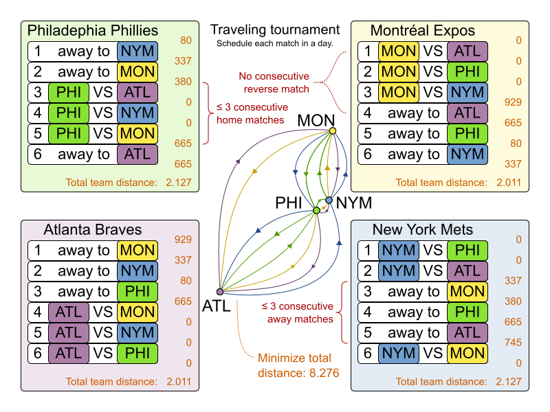
Hard constraints:
- Each team plays twice against every other team: once home and once away.
- Each team has exactly one match on each timeslot.
- No team must have more than three consecutive home or three consecutive away matches.
- No repeaters: no two consecutive matches of the same two opposing teams.
Soft constraints:
- Minimize the total distance traveled by all teams.
The problem is defined on Michael Trick’s website (which contains the world records too).
Problem size
1-nl04     has  6 days,  4 teams and   12 matches with a search space of    10^5.
1-nl06     has 10 days,  6 teams and   30 matches with a search space of   10^19.
1-nl08     has 14 days,  8 teams and   56 matches with a search space of   10^43.
1-nl10     has 18 days, 10 teams and   90 matches with a search space of   10^79.
1-nl12     has 22 days, 12 teams and  132 matches with a search space of  10^126.
1-nl14     has 26 days, 14 teams and  182 matches with a search space of  10^186.
1-nl16     has 30 days, 16 teams and  240 matches with a search space of  10^259.
2-bra24    has 46 days, 24 teams and  552 matches with a search space of  10^692.
3-nfl16    has 30 days, 16 teams and  240 matches with a search space of  10^259.
3-nfl18    has 34 days, 18 teams and  306 matches with a search space of  10^346.
3-nfl20    has 38 days, 20 teams and  380 matches with a search space of  10^447.
3-nfl22    has 42 days, 22 teams and  462 matches with a search space of  10^562.
3-nfl24    has 46 days, 24 teams and  552 matches with a search space of  10^692.
3-nfl26    has 50 days, 26 teams and  650 matches with a search space of  10^838.
3-nfl28    has 54 days, 28 teams and  756 matches with a search space of  10^999.
3-nfl30    has 58 days, 30 teams and  870 matches with a search space of 10^1175.
3-nfl32    has 62 days, 32 teams and  992 matches with a search space of 10^1367.
4-super04  has  6 days,  4 teams and   12 matches with a search space of    10^5.
4-super06  has 10 days,  6 teams and   30 matches with a search space of   10^19.
4-super08  has 14 days,  8 teams and   56 matches with a search space of   10^43.
4-super10  has 18 days, 10 teams and   90 matches with a search space of   10^79.
4-super12  has 22 days, 12 teams and  132 matches with a search space of  10^126.
4-super14  has 26 days, 14 teams and  182 matches with a search space of  10^186.
5-galaxy04 has  6 days,  4 teams and   12 matches with a search space of    10^5.
5-galaxy06 has 10 days,  6 teams and   30 matches with a search space of   10^19.
5-galaxy08 has 14 days,  8 teams and   56 matches with a search space of   10^43.
5-galaxy10 has 18 days, 10 teams and   90 matches with a search space of   10^79.
5-galaxy12 has 22 days, 12 teams and  132 matches with a search space of  10^126.
5-galaxy14 has 26 days, 14 teams and  182 matches with a search space of  10^186.
5-galaxy16 has 30 days, 16 teams and  240 matches with a search space of  10^259.
5-galaxy18 has 34 days, 18 teams and  306 matches with a search space of  10^346.
5-galaxy20 has 38 days, 20 teams and  380 matches with a search space of  10^447.
5-galaxy22 has 42 days, 22 teams and  462 matches with a search space of  10^562.
5-galaxy24 has 46 days, 24 teams and  552 matches with a search space of  10^692.
5-galaxy26 has 50 days, 26 teams and  650 matches with a search space of  10^838.
5-galaxy28 has 54 days, 28 teams and  756 matches with a search space of  10^999.
5-galaxy30 has 58 days, 30 teams and  870 matches with a search space of 10^1175.
5-galaxy32 has 62 days, 32 teams and  992 matches with a search space of 10^1367.
5-galaxy34 has 66 days, 34 teams and 1122 matches with a search space of 10^1576.
5-galaxy36 has 70 days, 36 teams and 1260 matches with a search space of 10^1801.
5-galaxy38 has 74 days, 38 teams and 1406 matches with a search space of 10^2042.
5-galaxy40 has 78 days, 40 teams and 1560 matches with a search space of 10^2301.
4.17. Cheap time scheduling
Schedule all tasks in time and on a machine to minimize power cost. Power prices differs in time. This is a form of job shop scheduling.
Hard constraints:
- Start time limits: Each task must start between its earliest start and latest start limit.
- Maximum capacity: The maximum capacity for each resource for each machine must not be exceeded.
- Startup and shutdown: Each machine must be active in the periods during which it has assigned tasks. Between tasks it is allowed to be idle to avoid startup and shutdown costs.
Medium constraints:
Power cost: Minimize the total power cost of the whole schedule.
- Machine power cost: Each active or idle machine consumes power, which infers a power cost (depending on the power price during that time).
- Task power cost: Each task consumes power too, which infers a power cost (depending on the power price during its time).
- Machine startup and shutdown cost: Every time a machine starts up or shuts down, an extra cost is inflicted.
Soft constraints (addendum to the original problem definition):
- Start early: Prefer starting a task sooner rather than later.
The problem is defined by the ICON challenge.
Problem size
sample01   has 3 resources,   2 machines, 288 periods and   25 tasks with a search space of    10^53.
sample02   has 3 resources,   2 machines, 288 periods and   50 tasks with a search space of   10^114.
sample03   has 3 resources,   2 machines, 288 periods and  100 tasks with a search space of   10^226.
sample04   has 3 resources,   5 machines, 288 periods and  100 tasks with a search space of   10^266.
sample05   has 3 resources,   2 machines, 288 periods and  250 tasks with a search space of   10^584.
sample06   has 3 resources,   5 machines, 288 periods and  250 tasks with a search space of   10^673.
sample07   has 3 resources,   2 machines, 288 periods and 1000 tasks with a search space of  10^2388.
sample08   has 3 resources,   5 machines, 288 periods and 1000 tasks with a search space of  10^2748.
sample09   has 4 resources,  20 machines, 288 periods and 2000 tasks with a search space of  10^6668.
instance00 has 1 resources,  10 machines, 288 periods and  200 tasks with a search space of   10^595.
instance01 has 1 resources,  10 machines, 288 periods and  200 tasks with a search space of   10^599.
instance02 has 1 resources,  10 machines, 288 periods and  200 tasks with a search space of   10^599.
instance03 has 1 resources,  10 machines, 288 periods and  200 tasks with a search space of   10^591.
instance04 has 1 resources,  10 machines, 288 periods and  200 tasks with a search space of   10^590.
instance05 has 2 resources,  25 machines, 288 periods and  200 tasks with a search space of   10^667.
instance06 has 2 resources,  25 machines, 288 periods and  200 tasks with a search space of   10^660.
instance07 has 2 resources,  25 machines, 288 periods and  200 tasks with a search space of   10^662.
instance08 has 2 resources,  25 machines, 288 periods and  200 tasks with a search space of   10^651.
instance09 has 2 resources,  25 machines, 288 periods and  200 tasks with a search space of   10^659.
instance10 has 2 resources,  20 machines, 288 periods and  500 tasks with a search space of  10^1657.
instance11 has 2 resources,  20 machines, 288 periods and  500 tasks with a search space of  10^1644.
instance12 has 2 resources,  20 machines, 288 periods and  500 tasks with a search space of  10^1637.
instance13 has 2 resources,  20 machines, 288 periods and  500 tasks with a search space of  10^1659.
instance14 has 2 resources,  20 machines, 288 periods and  500 tasks with a search space of  10^1643.
instance15 has 3 resources,  40 machines, 288 periods and  500 tasks with a search space of  10^1782.
instance16 has 3 resources,  40 machines, 288 periods and  500 tasks with a search space of  10^1778.
instance17 has 3 resources,  40 machines, 288 periods and  500 tasks with a search space of  10^1764.
instance18 has 3 resources,  40 machines, 288 periods and  500 tasks with a search space of  10^1769.
instance19 has 3 resources,  40 machines, 288 periods and  500 tasks with a search space of  10^1778.
instance20 has 3 resources,  50 machines, 288 periods and 1000 tasks with a search space of  10^3689.
instance21 has 3 resources,  50 machines, 288 periods and 1000 tasks with a search space of  10^3678.
instance22 has 3 resources,  50 machines, 288 periods and 1000 tasks with a search space of  10^3706.
instance23 has 3 resources,  50 machines, 288 periods and 1000 tasks with a search space of  10^3676.
instance24 has 3 resources,  50 machines, 288 periods and 1000 tasks with a search space of  10^3681.
instance25 has 3 resources,  60 machines, 288 periods and 1000 tasks with a search space of  10^3774.
instance26 has 3 resources,  60 machines, 288 periods and 1000 tasks with a search space of  10^3737.
instance27 has 3 resources,  60 machines, 288 periods and 1000 tasks with a search space of  10^3744.
instance28 has 3 resources,  60 machines, 288 periods and 1000 tasks with a search space of  10^3731.
instance29 has 3 resources,  60 machines, 288 periods and 1000 tasks with a search space of  10^3746.
instance30 has 4 resources,  70 machines, 288 periods and 2000 tasks with a search space of  10^7718.
instance31 has 4 resources,  70 machines, 288 periods and 2000 tasks with a search space of  10^7740.
instance32 has 4 resources,  70 machines, 288 periods and 2000 tasks with a search space of  10^7686.
instance33 has 4 resources,  70 machines, 288 periods and 2000 tasks with a search space of  10^7672.
instance34 has 4 resources,  70 machines, 288 periods and 2000 tasks with a search space of  10^7695.
instance35 has 4 resources,  80 machines, 288 periods and 2000 tasks with a search space of  10^7807.
instance36 has 4 resources,  80 machines, 288 periods and 2000 tasks with a search space of  10^7814.
instance37 has 4 resources,  80 machines, 288 periods and 2000 tasks with a search space of  10^7764.
instance38 has 4 resources,  80 machines, 288 periods and 2000 tasks with a search space of  10^7736.
instance39 has 4 resources,  80 machines, 288 periods and 2000 tasks with a search space of  10^7783.
instance40 has 4 resources,  90 machines, 288 periods and 4000 tasks with a search space of 10^15976.
instance41 has 4 resources,  90 machines, 288 periods and 4000 tasks with a search space of 10^15935.
instance42 has 4 resources,  90 machines, 288 periods and 4000 tasks with a search space of 10^15887.
instance43 has 4 resources,  90 machines, 288 periods and 4000 tasks with a search space of 10^15896.
instance44 has 4 resources,  90 machines, 288 periods and 4000 tasks with a search space of 10^15885.
instance45 has 4 resources, 100 machines, 288 periods and 5000 tasks with a search space of 10^20173.
instance46 has 4 resources, 100 machines, 288 periods and 5000 tasks with a search space of 10^20132.
instance47 has 4 resources, 100 machines, 288 periods and 5000 tasks with a search space of 10^20126.
instance48 has 4 resources, 100 machines, 288 periods and 5000 tasks with a search space of 10^20110.
instance49 has 4 resources, 100 machines, 288 periods and 5000 tasks with a search space of 10^20078.
4.18. Investment asset class allocation (Portfolio Optimization)
Decide the relative quantity to invest in each asset class.
Hard constraints:
Risk maximum: the total standard deviation must not be higher than the standard deviation maximum.
- Total standard deviation calculation takes asset class correlations into account by applying Markowitz Portfolio Theory.
- Region maximum: Each region has a quantity maximum.
- Sector maximum: Each sector has a quantity maximum.
Soft constraints:
- Maximize expected return.
Problem size
de_smet_1 has 1 regions, 3 sectors and 11 asset classes with a search space of 10^4.
irrinki_1 has 2 regions, 3 sectors and 6 asset classes with a search space of 10^3.
Larger datasets have not been created or tested yet, but should not pose a problem. A good source of data is this Asset Correlation website.
4.19. Conference scheduling
Assign each conference talk to a timeslot and a room. Timeslots can overlap. Read/write to/from an *.xlsx file that can be edited with LibreOffice or Excel too.
Hard constraints:
- Talk type of timeslot: The type of a talk must match the timeslot’s talk type.
- Room unavailable timeslots: A talk’s room must be available during the talk’s timeslot.
- Room conflict: Two talks can’t use the same room during overlapping timeslots.
- Speaker unavailable timeslots: Every talk’s speaker must be available during the talk’s timeslot.
- Speaker conflict: Two talks can’t share a speaker during overlapping timeslots.
Generic purpose timeslot and room tags
- Speaker required timeslot tag: If a speaker has a required timeslot tag, then all his/her talks must be assigned to a timeslot with that tag.
- Speaker prohibited timeslot tag: If a speaker has a prohibited timeslot tag, then all his/her talks cannot be assigned to a timeslot with that tag.
- Talk required timeslot tag: If a talk has a required timeslot tag, then it must be assigned to a timeslot with that tag.
- Talk prohibited timeslot tag: If a talk has a prohibited timeslot tag, then it cannot be assigned to a timeslot with that tag.
- Speaker required room tag: If a speaker has a required room tag, then all his/her talks must be assigned to a room with that tag.
- Speaker prohibited room tag: If a speaker has a prohibited room tag, then all his/her talks cannot be assigned to a room with that tag.
- Talk required room tag: If a talk has a required room tag, then it must be assigned to a room with that tag.
- Talk prohibited room tag: If a talk has a prohibited room tag, then it cannot be assigned to a room with that tag.
- Talk mutually-exclusive-talks tag: Talks that share such a tag must not be scheduled in overlapping timeslots.
- Talk prerequisite talks: A talk must be scheduled after all its prerequisite talks.
Soft constraints:
- Theme track conflict: Minimize the number of talks that share a same theme tag during overlapping timeslots.
- Sector conflict: Minimize the number of talks that share a same sector tag during overlapping timeslots.
- Content audience level flow violation: For every content tag, schedule the introductory talks before the advanced talks.
- Audience level diversity: For every timeslot, maximize the number of talks with a different audience level.
- Language diversity: For every timeslot, maximize the number of talks with a different language.
Generic purpose timeslot and room tags
- Speaker preferred timeslot tag: If a speaker has a preferred timeslot tag, then all his/her talks should be assigned to a timeslot with that tag.
- Speaker undesired timeslot tag: If a speaker has an undesired timeslot tag, then all his/her talks should not be assigned to a timeslot with that tag.
- Talk preferred timeslot tag: If a talk has a preferred timeslot tag, then it should be assigned to a timeslot with that tag.
- Talk undesired timeslot tag: If a talk has an undesired timeslot tag, then it should not be assigned to a timeslot with that tag.
- Speaker preferred room tag: If a speaker has a preferred room tag, then all his/her talks should be assigned to a room with that tag.
- Speaker undesired room tag: If a speaker has an undesired room tag, then all his/her talks should not be assigned to a room with that tag.
- Talk preferred room tag: If a talk has a preferred room tag, then it should be assigned to a room with that tag.
- Talk undesired room tag: If a talk has an undesired room tag, then it should not be assigned to a room with that tag.
- Same day talks: All talks that share a same theme tag or content tag should be scheduled in the minimum number of days (ideally in the same day).
Figure 4.14. Value proposition

Problem size
18talks-6timeslots-5rooms    has  18 talks,  6 timeslots and  5 rooms with a search space of  10^26.
36talks-12timeslots-5rooms   has  36 talks, 12 timeslots and  5 rooms with a search space of  10^64.
72talks-12timeslots-10rooms  has  72 talks, 12 timeslots and 10 rooms with a search space of 10^149.
108talks-18timeslots-10rooms has 108 talks, 18 timeslots and 10 rooms with a search space of 10^243.
216talks-18timeslots-20rooms has 216 talks, 18 timeslots and 20 rooms with a search space of 10^552.
4.20. Rock tour
Drive the rock bus from show to show, but schedule shows only on available days.
Hard constraints:
- Schedule every required show.
- Schedule as many shows as possible.
Medium constraints:
- Maximize revenue opportunity.
- Minimize driving time.
- Visit sooner than later.
Soft constraints:
- Avoid long driving times.
Problem size
47shows has 47 shows with a search space of 10^59.
4.21. Flight crew scheduling
Assign flights to pilots and flight attendants.
Hard constraints:
- Required skill: each flight assignment has a required skill. For example, flight AB0001 requires 2 pilots and 3 flight attendants.
- Flight conflict: each employee can only attend one flight at the same time
- Transfer between two flights: between two flights, an employee must be able to transfer from the arrival airport to the departure airport. For example, Ann arrives in Brussels at 10:00 and departs in Amsterdam at 15:00.
- Employee unavailability: the employee must be available on the day of the flight. For example, Ann is on PTO on 1-Feb.
Soft constraints:
- First assignment departing from home
- Last assignment arriving at home
- Load balance flight duration total per employee
Problem size
175flights-7days-Europe  has 2 skills, 50 airports, 150 employees, 175 flights and  875 flight assignments with a search space of  10^1904.
700flights-28days-Europe has 2 skills, 50 airports, 150 employees, 700 flights and 3500 flight assignments with a search space of  10^7616.
875flights-7days-Europe  has 2 skills, 50 airports, 750 employees, 875 flights and 4375 flight assignments with a search space of 10^12578.
175flights-7days-US      has 2 skills, 48 airports, 150 employees, 175 flights and  875 flight assignments with a search space of  10^1904.
Part II. Deploying and using the vehicle route planning starter application for Red Hat Business Optimizer
As a developer, you can use the OptaWeb Vehicle Routing starter application to optimize your vehicle fleet deliveries.
Prerequisites
- OpenJDK (JDK) 8 is installed. Red Hat build of Open JDK is available from the Software Downloads page in the Red Hat Customer Portal (login required).
- Apache Maven 3.6 or higher is installed. Maven is available from the Apache Maven Project website.
Chapter 5. What is OptaWeb Vehicle Routing?
The main purpose of many businesses is to transport various types of cargo. The goal of these businesses is to deliver a piece of cargo from the loading point to a destination and use its vehicle fleet in the most efficient way. One of the main objectives is to minimize travel costs which are measured in either time or distance.
This type of optimization problem is referred to as the vehicle routing problem (VRP) and has many variations.
Red Hat Business Optimizer can solve many of these vehicle routing variations and provides solution examples. Red Hat Business Optimizer enables developers to focus on modeling business rules and requirements instead of learning constraint programming theory. OptaWeb Vehicle Routing expands the vehicle routing capabilities of Red Hat Business Optimizer by providing a reference implementation that answers questions such as these:
- Where do I get the distances and travel times?
- How do I visualize the solution on a map?
- How do I build an application that runs in the cloud?
OptaWeb Vehicle Routing uses OpenStreetMap (OSM) data files. For information about OpenStreetMap, see the OpenStreetMap web site.
Use the following definitions when working with OptaWeb Vehicle Routing:
Region: An arbitrary area on the map of Earth, represented by an OSM file. A region can be a country, a city, a continent, or a group of countries that are frequently used together. For example, the DACH region includes Germany (DE), Austria (AT), and Switzerland (CH).
Country code: A two-letter code assigned to a country by the ISO-3166 standard. You can use a country code to filter geosearch results. Because you can work with a region that spans multiple countries (for example, the DACH region), OptaWeb Vehicle Routing accepts a list of country codes so that geosearch filtering can be used with such regions. For a list of country codes, see ISO 3166 Country Codes
Geosearch: A type of query where you provide an address or a place name of a region as the search keyword and receive a number of GPS locations as a result. The number of locations returned depends on how unique the search keyword is. Because most place names are not unique, filter out nonrelevant results by including only places in the country or countries that are in your working region.
Chapter 6. Download and build the OptaWeb Vehicle Routing deployment files
You must download and prepare the deployment files before building and deploying OptaWeb Vehicle Routing.
Procedure
Navigate to the Software Downloads page in the Red Hat Customer Portal (login required), and select the product and version from the drop-down options:
- Product: Red Hat Process Automation Manager
- Version: 7.10
-
Download Red Hat Process Automation Manager 7.10 Reference Implementations (
rhpam-7.10.0-reference-implementation.zip). -
Download Red Hat Process Automation Manager 7.10 Maven Repository (
rhpam-7.10.0-maven-repository.zip). -
Extract the
rhpam-7.10.0-maven-repository.zipfile. -
Copy the contents of the
rhpam-7.10.0-maven-repository/maven-repositorysubdirectory into the~/.m2/repositorydirectory. -
Extract the
rhpam-7.10.0-reference-implementation.zipfile. This archive contains three reference implementation ZIP files. -
Extract the
rhpam-7.10.0-optaweb-vehicle-routing.zipfile. -
Navigate to the
optaweb-vehicle-routing-distribution-7.48.0.Final-redhat-00004/sourcesdirectory. Enter the following command to build OptaWeb Vehicle Routing:
mvn clean package -DskipTests
Chapter 7. Run OptaWeb Vehicle Routing locally using the runLocally.sh script
Linux users can use the runLocally.sh Bash script to run OptaWeb Vehicle Routing.
The runLocally.sh script does not run on macOS. If you cannot use the runLocally.sh script, see Chapter 8, Configure and run OptaWeb Vehicle Routing manually.
The runLocally.sh script automates the following setup steps that otherwise must be carried out manually:
- Create the data directory.
- Download selected OpenStreetMap (OSM) files from Geofabrik.
- Try to associate a country code with each downloaded OSM file automatically.
- Build the project if the standalone JAR file does not exist.
- Launch OptaWeb Vehicle Routing by taking a single region argument or by selecting the region interactively.
See the following sections for instructions about executing the runLocally.sh script:
- Section 7.1, “Run the OptaWeb Vehicle Routing runLocally.sh script in quick start mode”
- Section 7.2, “Run the OptaWeb Vehicle Routing runLocally.sh script in interactive mode”
- Section 7.3, “Run the OptaWeb Vehicle Routing runLocally.sh script in non-interactive mode”
- Section 7.4, “Run the OptaWeb Vehicle Routing runLocally.sh script in air distance mode”
7.1. Run the OptaWeb Vehicle Routing runLocally.sh script in quick start mode
The easiest way to get started with OptaWeb Vehicle Routing is to run the runLocally.sh script without any arguments.
Prerequisites
- OptaWeb Vehicle Routing has been successfully built with Maven as described in Chapter 6, Download and build the OptaWeb Vehicle Routing deployment files.
- Internet access is available.
Procedure
Enter the following command in the
optaweb-vehicle-routing-distribution-7.48.0.Final-redhat-00004/sourcesdirectory../runLocally.sh
-
If prompted to create the
.optaweb-vehicle-routingdirectory, entery. You are prompted to create this directory the first time you run the script. If prompted to download an OSM file, enter
y. The first time that you run the script, OptaWeb Vehicle Routing downloads the Belgium OSM file.The application starts after the OSM file is downloaded.
To open the OptaWeb Vehicle Routing user interface, enter the following URL in a web browser:
http://localhost:8080
The first time that you run the script, it will take a few minutes to start because the OSM file must be imported by GraphHopper and stored as a road network graph. The next time you run the runlocally.sh script, load times will be significantly faster.
Next steps
7.2. Run the OptaWeb Vehicle Routing runLocally.sh script in interactive mode
Use interactive mode to see the list of downloaded OSM files and country codes assigned to each region. You can use the interactive mode to download additional OSM files from Geofabrik without visiting the website and choosing a destination for the download.
Prerequisites
- OptaWeb Vehicle Routing has been successfully built with Maven as described in Chapter 6, Download and build the OptaWeb Vehicle Routing deployment files.
- Internet access is available.
Procedure
-
Change directory to
optaweb-vehicle-routing-distribution-7.48.0.Final-redhat-00004/sources. Enter the following command to run the script in interactive mode:
./runLocally.sh -i
-
At the
Your choiceprompt, enterdto display the download menu. A list of previously downloaded regions appears followed by a list of regions that you can download. Optional: Select a region from the list of previously downloaded regions:
- Enter the number associated with a region in the list of downloaded regions.
- Press the Enter key.
Optional: Download a region:
-
Enter the number associated with the region that you want to download. For example, to select the map of Europe, enter
5. -
To download the map, enter
dthen press the Enter key. To download a specific region within the map, enter
ethen enter the number associated with the region that you want to download, and press the Enter key.Using large OSM filesFor the best user experience, use smaller regions such as individual European or US states. Using OSM files larger than 1 GB will require significant RAM size and take a lot of time (up to several hours) for the initial processing.
The application starts after the OSM file is downloaded.
-
Enter the number associated with the region that you want to download. For example, to select the map of Europe, enter
To open the OptaWeb Vehicle Routing user interface, enter the following URL in a web browser:
http://localhost:8080
Next steps
7.3. Run the OptaWeb Vehicle Routing runLocally.sh script in non-interactive mode
Use OptaWeb Vehicle Routing in non-interactive mode to start OptaWeb Vehicle Routing with a single command that includes an OSM file that you downloaded previously. This is useful when you want to switch between regions quickly or when doing a demo.
Prerequisites
- OptaWeb Vehicle Routing has been successfully built with Maven as described in Chapter 6, Download and build the OptaWeb Vehicle Routing deployment files.
- The OSM file for the region that you want to use has been downloaded. For information about downloading OSM files, see Section 7.2, “Run the OptaWeb Vehicle Routing runLocally.sh script in interactive mode”.
- Internet access is available.
Procedure
-
Change directory to
optaweb-vehicle-routing-distribution-7.48.0.Final-redhat-00004/sources. Execute the following command where
<OSM_FILE_NAME>is an OSM file that you downloaded previously:./runLocally.sh <OSM_FILE_NAME>
Next steps
7.4. Run the OptaWeb Vehicle Routing runLocally.sh script in air distance mode
OptaWeb Vehicle Routing can work in air distance mode that calculates travel times based on the distance between two coordinates. Use this mode in situations where you need to get OptaWeb Vehicle Routing up and running as quickly as possible and do not want to use an OSM (OpenStreetMap) file. Air distance mode is only useful if you need to smoke-test OptaWeb Vehicle Routing and you do not need accurate travel times.
Prerequisites
- OptaWeb Vehicle Routing has been successfully built with Maven as described in Chapter 6, Download and build the OptaWeb Vehicle Routing deployment files.
- Internet access is available.
Procedure
-
Change directory to
optaweb-vehicle-routing-distribution-7.48.0.Final-redhat-00004/sources. Run the
runLocally.shscript with the--airargument to start OptaWeb Vehicle Routing in air distance mode:./runLocally.sh --air
Next steps
7.5. Update the data directory
You can update the data directory that OptaWeb Vehicle Routing uses if you want to use a different data directory. The default data directory is $HOME/.optaweb-vehicle-routing.
Prerequisites
- OptaWeb Vehicle Routing has been successfully built with Maven as described in Chapter 6, Download and build the OptaWeb Vehicle Routing deployment files.
Procedure
-
To use a different data directory, at its absolute path to the
.DATA_DIR_LASTfile in the current data directory. To change country codes associated with a region, edit the corresponding file in the
country_codesdirectory, in the current data directory.For example, if you downloaded an OSM file for Scotland and the script fails to guess the country code, set the content of
country_codes/scotland-latestto GB.-
To remove a region, delete the corresponding OSM file from
openstreetmapdirectory in the data directory and delete the region’s directory in thegraphhopperdirectory.
Chapter 8. Configure and run OptaWeb Vehicle Routing manually
The easiest way to run OptaWeb Vehicle Routing is to use the runlocally.sh script. However, if Bash is not available on your system you can manually complete the steps that the runlocally.sh script performs.
Prerequisites
- OptaWeb Vehicle Routing has been successfully built with Maven as described in Chapter 6, Download and build the OptaWeb Vehicle Routing deployment files.
- Internet access is available.
Procedure
Download routing data.
The routing engine requires geographical data to calculate the time it takes vehicles to travel between locations. You must download and store OpenStreetMap (OSM) data files on the local file system before you run OptaWeb Vehicle Routing.
NoteThe OSM data files are typically between 100 MB to 1 GB and take time to download so it is a good idea to download the files before building or starting the OptaWeb Vehicle Routing application.
-
Open
http://download.geofabrik.de/in a web browser. - Click a region in the Sub Region list, for example Europe. The subregion page opens.
-
In the Sub Regions table, download the OSM file (
.osm.pbf) for a country, for example Belgium.
-
Open
Create the data directory structure.
OptaWeb Vehicle Routing reads and writes several types of data on the file system. It reads OSM (OpenStreetMap) files from the
openstreetmapdirectory, writes a road network graph to thegraphhopperdirectory, and persists user data in a directory calleddb. Create a new directory dedicated to storing all of these data to make it easier to upgrade to a newer version of OptaWeb Vehicle Routing in the future and continue working with the data you created previously.-
Create the
$HOME/{VRP-DATA-DIR}directory. Create the
openstreetmapdirectory in the$HOME/{VRP-DATA-DIR}directory:$HOME/{VRP-DATA-DIR} └── openstreetmapMove all of your downloaded OSM files (files with the extension
.osm.pbf) to theopenstreetmapdirectory.The rest of the directory structure is created by the OptaWeb Vehicle Routing application when it runs for the first time. After that, your directory structure is similar to the following example:
$HOME/{VRP-DATA-DIR}

├── db
│   └── vrp.mv.db
├── graphhopper
│   └── belgium-latest
└── openstreetmap
    └── belgium-latest.osm.pbf
-
Create the
-
Change directory to
optaweb-vehicle-routing-distribution-7.48.0.Final-redhat-00004/sources/optaweb-vehicle-routing-standalone/target. To run OptaWeb Vehicle Routing, enter the following command:
java -jar optaweb-vehicle-routing-standalone-7.48.0.Final-redhat-00004.jar \
--app.persistence.h2-dir=$HOME/{VRP-DATA-DIR}/db \
--app.routing.gh-dir=$HOME/{VRP-DATA-DIR}/graphhopper \
--app.routing.osm-dir=$HOME/{VRP-DATA-DIR}/openstreetmap \
--app.routing.osm-file=<OSM_FILE_NAME> \
--app.region.country-codes=<COUNTRY_CODE_LIST> \
In this command, replace the following variables:
-
<OSM_FILE_NAME>: The OSM file for the region that you want to use and that you downloaded previously <COUNTRY_CODE_LIST>: A comma-separated list of country codes used to filter geosearch queries. For a list of country codes, see ISO 3166 Country Codes.The application starts after the OSM file is downloaded.
In the following example, OptaWeb Vehicle Routing downloads the OSM map of Central America (
central-america-latest.osm.pbf) and searches in the countries Belize (BZ) and Guatemala (GT).java -jar optaweb-vehicle-routing-standalone-7.48.0.Final-redhat-00004.jar \ --app.persistence.h2-dir=/home/user/.optaweb-vehicle-routing/db \ --app.routing.osm-dir=/home/user/.optaweb-vehicle-routing/openstreetmap \ --app.routing.gh-dir=/home/user/.optaweb-vehicle-routing/graphhopper \ --app.routing.osm-file=central-america-latest.osm.pbf \ --app.region.country-codes=BZ,GT
-
To open the OptaWeb Vehicle Routing user interface, enter the following URL in a web browser:
http://localhost:8080
Next steps
Chapter 9. Run OptaWeb Vehicle Routing on Red Hat OpenShift Container Platform
Linux users can use the runOnOpenShift.sh Bash script to install OptaWeb Vehicle Routing on Red Hat OpenShift Container Platform.
The runOnOpenShift.sh script does not run on macOS.
Prerequisites
-
You have access to an OpenShift cluster and the OpenShift command-line interface (
oc) has been installed. For information about Red Hat OpenShift Container Platform, see Installing OpenShift Container Platform. - OptaWeb Vehicle Routing has been successfully built with Maven as described in Chapter 6, Download and build the OptaWeb Vehicle Routing deployment files.
- Internet access is available.
Procedure
- Log in to or start a Red Hat OpenShift Container Platform cluster.
Enter the following command where
<PROJECT_NAME>is the name of your new project:oc new-project <PROJECT_NAME>
-
If necessary, change directory to
optaweb-vehicle-routing-distribution-7.48.0.Final-redhat-00004/sources. Enter the following command to execute the
runOnOpenShift.shscript and download an OpenStreetMap (OSM) file:./runOnOpenShift.sh <OSM_FILE_NAME> <COUNTRY_CODE_LIST> <OSM_FILE_DOWNLOAD_URL>
In this command, replace the following variables:
-
<OSM_FILE_NAME>: The name of a file downloaded from<OSM_FILE_DOWNLOAD_URL>. -
<COUNTRY_CODE_LIST>: A comma-separated list of country codes used to filter geosearch queries. For a list of country codes, see ISO 3166 Country Codes. <OSM_FILE_DOWNLOAD_URL>: The URL of an OSM data file in PBF format accessible from OpenShift. The file will be downloaded during backend startup and saved as/deployments/local/<OSM_FILE_NAME>.The following example configures OptaWeb Vehicle Routing to filter geosearch results to Belgium and downloads the latest Belgium OSM extract from Geofabrik:
In the following example, OptaWeb Vehicle Routing downloads the OSM map of Central America (
central-america-latest.osm.pbf) and searches in the countries Belize (BZ) and Guatemala (GT)../runOnOpenShift.sh central-america-latest.osm.pbf BZ,GT http://download.geofabrik.de/europe/central-america-latest.osm.pbf
-
For help with the runOnOpenShift.sh script, enter ./runOnOpenShift.sh --help.
9.1. Updating the deployed OptaWeb Vehicle Routing application with local changes
After you deploy your OptaWeb Vehicle Routing application on Red Hat OpenShift Container Platform, you can update the back end and front end.
Prerequisites
- OptaWeb Vehicle Routing has been successfully built with Maven and deployed on OpenShift.
Procedure
To update the back end, perform the following steps:
- Change the source code and build the back end module with Maven.
-
Change directory to
optaweb-vehicle-routing-distribution-7.48.0.Final-redhat-00004/sources/optaweb-vehicle-routing-backend. Enter the following command to start the OpenShift build:
oc start-build backend --from-dir=. --follow
To update the front end, perform the following steps:
-
Change the source code and build the front end module with the
npmutility. -
Change directory to
sources/optaweb-vehicle-routing-frontend. Enter the following command to start the OpenShift build:
oc start-build frontend --from-dir=docker --follow
-
Change the source code and build the front end module with the
Next steps
Chapter 10. Using OptaWeb Vehicle Routing
In the OptaWeb Vehicle Routing application, you can mark a number of locations on the map. The first location is assumed to be the depot. Vehicles must deliver goods from this depot to every other location that you marked.
You can set the number of vehicles and the carrying capacity of every vehicle. However, the route is not guaranteed to use all vehicles. The application uses as many vehicles as required for an optimal route.
The current version has certain limitations:
- Every delivery to a location is supposed to take one point of vehicle capacity. For example, a vehicle with a capacity of 10 can visit up to 10 locations before returning to the depot.
- Setting custom names of vehicles and locations is not supported.
10.1. Creating a route
To create an optimal route, use the Demo tab of the OptaWeb Vehicle Routing user interface.
Prerequisites
- OptaWeb Vehicle Routing is running and you have access to the user interface.
Procedure
- In OptaWeb Vehicle Routing, click Demo to open the Demo tab.
- Use the blue minus and plus buttons above the map to set the number of vehicles. Each vehicle has a default capacity of 10.
Use the plus button in a square on the map to zoom in as required.
NoteDo not double-click to zoom in. A double click also creates a location.
- Click a location for the depot.
- Click other locations on the map for delivery points.
If you want to delete a location:
- Hover the mouse cursor over the location to see the location name.
- Find the location name in the list in the left part of the screen.
- Click the X icon next to the name.
Every time you add or remove a location or change the number of vehicles, the application creates and displays a new optimal route. If the solution uses several vehicles, the application shows the route for every vehicle in a different color.
10.2. Viewing and setting other details
You can use other tabs in OptaWeb Vehicle Routing user interface to view and set additional details.
Prerequisites
- OptaWeb Vehicle Routing is running and you have access to the user interface.
Procedure
- Click the Vehicles tab to view, add, and remove vehicles, and also set the capacity for every vehicle.
- Click the Visits tab to view and remove locations.
- Click the Route tab to select each vehicle and view the route for the selected vehicle.
10.3. Creating custom data sets with OptaWeb Vehicle Routing
There is a built-in demo data set consisting of a several large Belgian cities. If you want to have more demos available in the Load demo menu, you can prepare your own data sets.
Procedure
To do that, follow these steps:
- In OptaWeb Vehicle Routing, add a depot and a number of visits by clicking on the map or using geosearch.
Click Export and save the file in the data set_directory.
NoteThe data set directory is the directory specified in the
app.demo.data-set-dirproperty.If the application is running through the
runLocally.shscript, the data set directory is set to$HOME/{VRP-DATA-DIR}/dataset.Otherwise, the property is from
application.propertiesand defaults tooptaweb-vehicle-routing-distribution-7.48.0.Final-redhat-00004/sources/optaweb-vehicle-routing-standalone/target/local/dataset.You can edit the
app.demo.data-set-dirproperty to specify a diffent data directory.- Edit the YAML file and choose a unique name for the data set.
- Restart the back end.
After you restart the back end, files in the data set directory appear in the Load demo menu.
10.4. Troubleshooting OptaWeb Vehicle Routing
If the OptaWeb Vehicle Routing behaves unexpectedly, follow this procedure to trouble-shoot.
Prerequisites
- OptaWeb Vehicle Routing is running and behaving unexpectedly.
Procedure
- To identify issues, review the back end terminal output log.
To resolve issues, remove the back end database:
- Stop the back end by pressing kbd:[Ctrl+C] in the back end terminal window.
-
Remove the directory
optaweb-vehicle-routing/optaweb-vehicle-routing-backend/local/db. - Restart OptaWeb Vehicle Routing.
Chapter 11. OptaWeb Vehicle Routing development guide
This section describes how to configure and run the back and front end modules in development mode.
11.1. OptaWeb Vehicle Routing project structure
The OptaWeb Vehicle Routing project is a multi-module Maven project.
Figure 11.1. Module dependency tree diagram
The back end and front end modules are at the bottom of the module tree. These modules contain the application source code.
The standalone module is an assembly module that combines the back end and front end into a single executable JAR file.
The distribution module represents the final assembly step. It takes the standalone application and the documentation and wraps them in an archive that is easy to distribute.
The back end and front end are separate projects that you can build and deploy separately. In fact, they are written in completely different languages and built with different tools. Both projects have tools that provide a modern developer experience with fast turn-around between code changes and the running application.
The next sections describe how to run both back end and front end projects in development mode.
11.2. The OptaWeb Vehicle Routing back end module
The back end module contains a server-side application that uses Red Hat Business Optimizer to optimize vehicle routes. Optimization is a CPU-intensive computation that must avoid any I/O operations in order to perform to its full potential. Because one of the chief objectives is to minimize travel cost, either time or distance, OptaWeb Vehicle Routing keeps the travel cost information in RAM memory. While solving, Red Hat Business Optimizer needs to know the travel cost between every pair of locations entered by the user. This information is stored in a structure called the distance matrix.
When you enter a new location, OptaWeb Vehicle Routing calculates the travel cost between the new location and every other location that has been entered so far, and stores the travel cost in the distance matrix. The travel cost calculation is performed by the GraphHopper routing engine.
The back end module implements the following additional supporting functionality:
- Persistence
- WebSocket connection for the front end
- Data set loading, export, and import
To learn more about the back end code architecture, see Chapter 12, OptaWeb Vehicle Routing back end architecture.
The next sections describe how to configure and run the back end in development mode.
11.2.1. Running the OptaWeb Vehicle Routing back end module using the Spring Boot Maven plugin
You can use the Spring Boot plug-in to run the OptaWeb Vehicle Routing back end module in development mode.
Prerequisites
- OptaWeb Vehicle Routing has been configured as described in Chapter 8, Configure and run OptaWeb Vehicle Routing manually.
Procedure
-
Change directory to
optaweb-vehicle-routing-distribution-7.48.0.Final-redhat-00004/sources/optaweb-vehicle-routing-backend. To run the back end in development mode, enter the following command:
mvn spring-boot:run
11.2.2. Running the OptaWeb Vehicle Routing back end module from IntelliJ IDEA
You can use the IntelliJ IDEA to run the OptaWeb Vehicle Routing back end module to make it easier to develop your project.
Procedure
In IntelliJ IDEA, enter
org.optaweb.vehiclerouting.OptaWebVehicleRoutingApplication. This creates a run configuration that you will edit in the next step.-
Open the
OptaWebVehicleRoutingApplicationclass in the Editor window. Click the green symbol in the editor window gutter and select Run OptaWebVehicleRoutingApplication. The run fails because the working directory is set to the root of the project where the back end module directory is expected.
NoteSee the Run Applications page on the IntelliJ IDEA web site to learn more about running applications in IntelliJ IDEA.
-
Open the
- Select Run→Edit Configurations and then select Spring Boot→OptaWebVehicleRoutingApplication.
-
Set Program arguments to
--spring.profiles.active=localto activate the Spring profile calledlocal. This directs the application to use configurations in theapplication-local.propertiesfile. -
Change Working directory to the back end module (
optaweb-vehicle-routing-backend). Set On Update action to Hot swap classes and update trigger file if failed. This enables you to use the Update action to quickly restart the application.
For more information, see Spring and Spring Boot in IntelliJ IDEA 2018.1.
11.2.3. Spring Boot automatic restart
Automatic restart is provided by Spring Boot DevTools. When you run the OptaWeb Vehicle Routing back end with the Spring Boot Maven plug-in, the application automatically restarts whenever files on the classpath change. Automatic restart scans files on the classpath, so you only need to recompile your changes to trigger application restart. No IDE configuration is needed.
If your IDE has a compile-on-save feature (for example Eclipse or NetBeans), you just need to save the files that have changed since the last compilation.
IntelliJ IDEA saves changes automatically and you need to select either Build[Recompile], which recompiles the file in the active tab, or Build[Build Project] which recompiles all changes. For more information, see Compile and build applications with IntelliJ IDEA.
11.2.4. Setting OptaWeb Vehicle Routing back end module configuration properties
There are several ways that you can set OptaWeb Vehicle Routing back end module configuration properties. The methods in this section are useful if you are running OptaWeb Vehicle Routing locally.
Prerequisites
- The OptaWeb Vehicle Routing reference implementation has been downloaded and extracted. For information, see Chapter 6, Download and build the OptaWeb Vehicle Routing deployment files.
Procedure
-
Set configuration properties in the
application.propertiesfile: -
Change directory to
rhpam-7.48.0.Final-redhat-00004-optaweb-vehicle-routing/sources/optaweb-vehicle-routing-backend/src/main/resources. -
Open the
application.propertiesfile in a text editor. Edit or add properties and then save the file.
Use a command line argument when running the packaged application. In the following example,
<PROPERTY>is the name of a property and<VALUE>is the value of that property:java -jar optaweb-vehicle-routing-backend.jar --app.<PROPERTY>=<VALUE>
Use an environment variable when running the application with
spring-boot:run:<PROPERTY>=<VALUE> ./mvnw spring-boot:run
NoteThis method requires relaxed binding which only works if the property is defined using
@ConfigurationProperties.
It is not possible to set properties by specifying -D when running the application using the Spring Boot Maven plugin (./mvnw spring-boot:run -D<PROPERTY). Any system properties to be set by the plugin to the forked Java process in which the application runs must be specified in the pom.xml file using the systemPropertiesVariables attribute. For information about this attribute, see Using System Properties on the Spring web site.
You can learn more about configuring a Spring Boot application on the Spring Boot Externalized Configuration page.
Use src/main/resources/application-local.properties to store your personal configuration without affecting the Git working tree.
For a complete list of OptaWeb Vehicle Routing configuration properties, see Chapter 13, OptaWeb Vehicle Routing back end configuration properties.
For a complete list of application properties available in Spring Boot, see the Common Application Properties page on the Spring web site.
11.2.5. OptaWeb Vehicle Routing backend logging
OptaWeb Vehicle Routing uses the SLF4J API and Logback as the logging framework. The Spring environment enables you to configure most logging aspects, including levels, patterns, and log files, in the same way as other configuration properties. The most common ways to set logging properties are by editing the application.properties file or using arguments such as <PROPERTY>=<VALUE> where <PROPERTY> is the name of a property and <VALUE> is the value of that property. See the Spring Boot Logging documentation for more information.
The following examples are properties that you can use to control logging level of some parts of the application:
-
logging.level.org.optaweb.vehiclerouting=debug: Enables the debug level for the back end code -
logging.level.org.optaplanner.core=warn: Reduces Red Hat Business Optimizer logging -
logging.level.org.springframework.web.socket=trace: Accesses more details when investigating problems with WebSocket connection
11.3. Working with the OptaWeb Vehicle Routing front end module
The front end project was bootstrapped with Create React App. Create React App provides a number of scripts and dependencies that help with development and with building the application for production.
Prerequisites
- The OptaWeb Vehicle Routing reference implementation has been downloaded and extracted. For information, see Chapter 6, Download and build the OptaWeb Vehicle Routing deployment files.
Procedure
On Fedora, enter the following command to set up the development environment:
sudo dnf install npm
See Downloading and installing Node.js and npm for more information about installing npm.
-
Change directory to
optaweb-vehicle-routing-distribution-7.48.0.Final-redhat-00004/sources/optaweb-vehicle-routing-frontend. Install
npmdependencies:npm install
Unlike Maven, the
npmpackage manager installs dependencies innode_modulesunder the project directory and does that only when you executenpm install. Whenever the dependencies listed inpackage.jsonchange, for example when you pull changes to the master branch, you must executenpm installbefore you run the development server.Enter the following command to run the development server:
npm start
If it does not open automatically, open
http://localhost:3000/in a web browser.By default, the
npm startcommand attempts to open this URL in your default browser.NoteIf you do not want the
npm startcommand to open a new browser tab each time you run it, export theBROWSER=noneenvironment variable. You can use.env.localfile to make this preference permanent. To do that, enter the following command:echo BROWSER=none >> .env.local
The browser refreshes the page whenever you make changes in the front end source code. The development server process running in the terminal picks up the changes as well and prints compilation and lint errors to the console.
Enter the following command to run tests:
npm test
Change the value of the
REACT_APP_BACKEND_URLenvironment variable to specify the location of the back end project to be used bynpmwhen you executenpm startornpm run build, for example:REACT_APP_BACKEND_URL=http://10.0.0.123:8081
NoteEnvironment variables are hard coded inside the JavaScript bundle during the
npmbuild process, so you must specify the back end location before you build and deploy the front end.To learn more about the React environment variables, see Adding Custom Environment Variables.
To build the front end, enter one of the following commands:
./mvnw install
mvn install
Chapter 12. OptaWeb Vehicle Routing back end architecture
Domain model and use cases are essential for the application. The OptaWeb Vehicle Routing domain model is at the center of the architecture and is surround by the application layer that embeds use cases. Functions such as route optimization, distance calculation, persistence, and network communication are considered implementation details and are placed at the outermost layer of the architecture.
Figure 12.1. Diagram of application layers
12.1. Code organization
The back end code is organized in three layers, illustrated in the preceding graphic.
org.optaweb.vehiclerouting
├── domain
├── plugin          # Infrastructure layer
│   ├── persistence
│   ├── planner
│   ├── routing
│   └── websocket
└── service         # Application layer
    ├── demo
    ├── distance
    ├── location
    ├── region
    ├── reload
    ├── route
    └── vehicle
The service package contains the application layer that implements use cases. The plugin package contains the infrastructure layer.
Code in each layer is further organized by function. This means that each service or plug-in has its own package.
12.2. Dependency rules
Compile-time dependencies are only allowed to point from outer layers towards the center. Following this rule helps to keep the domain model independent of underlying frameworks and other implementation details and models the behavior of business entities more precisely. With presentation and persistence being pushed out to the periphery, it is easier to test the behavior of business entities and use cases.
The domain has no dependencies.
Services only depend on the domain. If a service needs to send a result (for example to the database or to the client), it uses an output boundary interface. Its implementation is injected by the Inversion of Control (IoC) container.
Plug-ins depend on services in two ways. First, they invoke services based on events such as a user input or a route update coming from the optimization engine. Services are injected into plug-ins which moves the burden of their construction and dependency resolution to the IoC container. Second, plug-ins implement service output boundary interfaces to handle use case results, for example persisting changes to the database or sending a response to the web UI.
12.3. The domain package
The domain package contains business objects that model the domain of this project, for example Location, Vehicle, Route. These objects are strictly business-oriented and must not be influenced by any tools and frameworks, for example object-relational mapping tools and web service frameworks.
12.4. The service package
The service package contains classes that implement use cases. A use case describes something that you want to do, for example adding a new location, changing vehicle capacity, or finding coordinates for an address. The business rules that govern use cases are expressed using the domain objects.
Services often need to interact with plug-ins in the outer layer, such as persistence, web, and optimization. To satisfy the dependency rules between layers, the interaction between services and plug-ins is expressed in terms of interfaces that define the dependencies of a service. A plug-in can satisfy a dependency of a service by providing a bean that implements the boundary interface of the service. The Spring IoC container creates an instance of the plug-in bean and injects it to the service at runtime. This is an example of the inversion of control principle.
12.5. The plugin package
The plugin package contains infrastructure functions such as optimization, persistence, routing, and network.
Chapter 13. OptaWeb Vehicle Routing back end configuration properties
You can set the OptaWeb Vehicle Routing application properties listed in the following table.
| Property | Type | Example | Description |
|---|---|---|---|
|
| Relative or absolute path |
|
Custom data sets are loaded from this directory. Defaults to |
|
| Relative or absolute path |
|
The directory used by H2 to store the database file. Defaults to |
|
|
List of |
| Restricts geosearch results. |
|
| Enumeration |
|
Routing engine implementation. Defaults to |
|
| Relative or absolute path |
|
The directory used by GraphHopper to store road network graphs. Defaults to |
|
| Relative or absolute path |
|
The directory that contains OSM files. Defaults to |
|
| File name |
|
Name of the OSM file to be loaded by GraphHopper. The file must be placed under |
|
|
|
| How long the solver should run after a location change occurs. |
|
| IP address or hostname |
| Network address to which to bind the server. |
|
| Port number |
| Server HTTP port. |
Part III. Running and modifying the employee rostering starter application for Red Hat Business Optimizer using an IDE
As a business rules developer, you can use an IDE to build, run, and modify the optaweb-employee-rostering starter application that uses the Red Hat Business Optimizer functionality.
Prerequisites
- You use an integrated development environment, such as Red Hat CodeReady Studio or IntelliJ IDEA.
- You have an understanding of the Java language.
- You have an understanding of React and TypeScript. This requirement is necessary to develop the OptaWeb UI.
Chapter 14. Overview of the employee rostering starter application
The employee rostering starter application assigns employees to shifts on various positions in an organization. For example, you can use the application to distribute shifts in a hospital between nurses, guard duty shifts across a number of locations, or shifts on an assembly line between workers.
Optimal employee rostering must take a number of variables into account. For example, different skills can be required for shifts in different positions. Also, some employees might be unavailable for some time slots or might prefer a particular time slot. Moreover, an employee can have a contract that limits the number of hours that the employee can work in a single time period.
The Red Hat Business Optimizer rules for this starter application use both hard and soft constraints. During an optimization, the planning engine may not violate hard constraints, for example, if an employee is unavailable (out sick), or that an employee cannot work two spots in a single shift. The planning engine tries to adhere to soft constraints, such as an employee’s preference to not work a specific shift, but can violate them if the optimal solution requires it.
Chapter 15. Building and running the employee rostering starter application
You can build the employee rostering starter application from the source code and run it as a JAR file.
Alternatively, you can use your IDE, for example, Eclipse (including Red Hat CodeReady Studio), to build and run the application.
15.1. Preparing deployment files
You must download and prepare the deployment files before building and deploying the application.
Procedure
-
Download the
rhpam-7.10.0-reference-implementation.zipfile from the Software Downloads page for Red Hat Process Automation Manager 7.10. - Unzip the downloaded archive.
-
Copy the contents of the
jboss-rhba-7.10.0.GA-maven-repository/maven-repositorysubdirectory into the~/.m2/repositorydirectory. Expand the
rhpam-7.10.0-optaweb-employee-rostering.zipfile that is extracted from the reference implementation archive.The
optaweb-employee-rostering-distribution-7.48.0.Final-redhat-00004folder is created. This folder is the base folder in subsequent parts of this document.NoteFile and folder names might have higher version numbers than specifically noted in this document.
15.2. Running the Employee Rostering starter application JAR file
You can run the Employee Rostering starter application from a JAR file included in the reference implementation download.
Prerequisites
-
You have downloaded and extracted the
rhpam-7.10.0-reference-implementation.zipfile as described in Section 15.1, “Preparing deployment files”. - A Java Development Kit is installed.
- Maven is installed.
- The host has access to the Internet. The build process uses the Internet for downloading Maven packages from external repositories.
Procedure
-
In a command terminal, change to the
sourcesdirectory. Enter the following command:
mvn clean install -DskipTests
- Wait for the build process to complete.
-
Navigate to the
optaweb-employee-rostering-distribution-7.48.0.Final-redhat-00004/sources/optaweb-employee-rostering-standalone/targetdirectory. Enter the following command to run the Employee Rostering JAR file:
java -jar optaweb-employee-rostering-standalone-*-exec.jar
NoteThis command starts the employee rostering application with a non-production database. To start the employee rostering application with a production database, add the
--spring.profiles.active=productionargument to the preceding command.-
To access the application, enter
http://localhost:8080/in a web browser.
15.3. Building and running the Employee Rostering starter application using Maven
You can use the command line to build and run the employee rostering starter application.
If you use this procedure, the data is stored in memory and is lost when the server is stopped. To build and run the application with a database server for persistent storage, see Section 15.4, “Building and running the employee rostering starter application with persistent data storage from the command line”.
Prerequisites
- You prepared the deployment files as described in Section 15.1, “Preparing deployment files”.
- A Java Development Kit is installed.
- Maven is installed.
- The host has access to the Internet. The build process uses the Internet for downloading Maven packages from external repositories.
Procedure
-
Navigate to the
optaweb-employee-rostering-backenddirectory. Enter the following command:
mvn spring-boot:run
-
Navigate to the
optaweb-employee-rostering-frontenddirectory. Enter the following command:
npm start
NoteIf you use
npmto start the server,npmmonitors code changes.-
To access the application, enter
http://localhost:3000/in a web browser.
15.4. Building and running the employee rostering starter application with persistent data storage from the command line
If you use the command line to build the employee rostering starter application and run it, you can provide a database server for persistent data storage.
Prerequisites
- You prepared the deployment files as described in Section 15.1, “Preparing deployment files”.
- A Java Development Kit is installed.
- Maven is installed.
- The host has access to the Internet. The build process uses the Internet for downloading Maven packages from external repositories.
- You have a deployed MySQL or PostrgeSQL database server.
Procedure
-
In a command terminal, navigate to the
optaweb-employee-rostering-standalone/targetdirectory. Enter the following command to run the Employee Rostering JAR file:
java -jar optaweb-employee-rostering-standalone-*-exec.jar --spring.profiles.active=production
spring.datasource.url=<DATABASE_URL> --spring.datasource.username=<DATABASE_USER> --spring.datasource.password=<DATABASE_PASSWORD>
In this example, replace the following placeholders:
-
<DATABASE_URL>: URL to connect to the database, for examplejdbc:postgresql://postgresql:5432/MY_DATABASE -
<DATABASE_USER>: The user to connect to the database -
<DATABASE_PASSWORD>: The password for<DATABASE_USER>
-
15.5. Building and running the employee rostering starter application using IntelliJ IDEA
You can use IntelliJ IDEA to build and run the employee rostering starter application.
Prerequisites
- You have downloaded the Employee Rostering source code, available from the Employee Rostering GitHub page.
- IntelliJ IDEA, Maven, and Node.js are installed.
- The host has access to the Internet. The build process uses the Internet for downloading Maven packages from external repositories.
Procedure
- Start IntelliJ IDEA.
- From the IntelliJ IDEA main menu, select File → Open.
- Select the root directory of the application source and click OK.
- From the main menu, select Run → Edit Configurations.
- In the window that appears, expand Templates and select Maven. The Maven sidebar appears.
-
In the Maven sidebar, select
optaweb-employee-rostering-backendfrom the Working Directory menu. -
In Command Line, enter
spring-boot:run. - To start the back end, click OK .
-
In a command terminal, navigate to the
optaweb-employee-rostering-frontenddirectory. Enter the following command to start the front end:
npm start
-
To access the application, enter
http://localhost:3000/in a web browser.
Chapter 16. Overview of the source code of the employee rostering starter application
The employee rostering starter application consists of the following principal components:
-
A
backendthat implements the rostering logic using Red Hat Business Optimizer and provides a REST API -
A
frontendmodule that implements a user interface using React and interacts with thebackendmodule through the REST API
You can build and use these components independently. In particular, you can implement a different user interface and use the REST API to call the server.
In addition to the two main components, the employee rostering template contains a generator of random source data (useful for demonstration and testing purposes) and a benchmarking application.
Modules and key classes
The Java source code of the employee rostering template contains several Maven modules. Each of these modules includes a separate Maven project file (pom.xml), but they are intended for building in a common project.
The modules contain a number of files, including Java classes. This document lists all the modules, as well as the classes and other files that contain the key information for the employee rostering calculations.
-
optaweb-employee-rostering-benchmarkmodule: Contains an additional application that generates random data and benchmarks the solution. -
optaweb-employee-rostering-distributionmodule: Contains README files. -
optaweb-employee-rostering-docsmodule: Contains documentation files. -
optaweb-employee-rostering-frontendmodule: Contains the client application with the user interface, developed in React. optaweb-employee-rostering-backendmodule: Contains the server application that uses Red Hat Business Optimizer to perform the rostering calculation.-
src/main/java/org.optaweb.employeerostering.service.roster/rosterGenerator.java: Generates random input data for demonstration and testing purposes. If you change the required input data, change the generator accordingly. -
src/main/java/org.optaweb.employeerostering.domain.employee/EmployeeAvailability.java: Defines availability information for an employee. For every time slot an employee can be unavailable, available, or it can be designated a preferred time slot for the employee. -
src/main/java/org.optaweb.employeerostering.domain.employee/Employee.java: Defines an employee. An employee has a name, a list of skills, and works under a contract. Skills are represented by skill objects. -
src/main/java/org.optaweb.employeerostering.domain.roster/Roster.java: Defines the calculated rostering information. -
src/main/java/org.optaweb.employeerostering.domain.shift/Shift.java: Defines a shift to which an employee can be assigned. A shift is defined by a time slot and a spot. For example, in a diner there could be a shift in the Kitchen spot for the February 20 8AM-4PM time slot. Multiple shifts can be defined for a given spot and time slot. In this case, multiple employees are required for this spot and time slot. -
src/main/java/org.optaweb.employeerostering.domain.skill/Skill.java: Defines a skill that an employee can have. -
src/main/java/org.optaweb.employeerostering.domain.spot/Spot.java: Defines a spot where employees can be placed. For example, aKitchencan be a spot. -
src/main/java/org.optaweb.employeerostering.domain.contract/Contract.java: Defines a contract that sets limits on work time for an employee in various time periods. -
src/main/java/org.optaweb.employeerostering.domain.tenant/Tenant.java: Defines a tenant. Each tenant represents an independent set of data. Changes in the data for one tenant do not affect any other tenants. -
*View.java: Classes related to domain objects that define value sets that are calculated from other information; the client application can read these values through the REST API, but not write them. -
*Service.java: Interfaces located in the service package that define the REST API. Both the server and the client application separately define implementations of these interfaces.
-
Chapter 17. Modifying the employee rostering starter application
To modify the employee rostering starter application to suit your needs, you must change the rules that govern the optimization process. You must also ensure that the data structures include the required data and provide the required calculations for the rules. If the required data is not present in the user interface, you must also modify the user interface.
The following procedure outlines the general approach to modifying the employee rostering starter application.
Prerequisites
- You have a build environment that successfully builds the application.
- You can read and modify Java code.
Procedure
Plan the required changes. Answer the following questions:
- What are the additional scenarios that must be avoided? These scenarios are hard constraints.
- What are the additional scenarios that the optimizer must try to avoid when possible? These scenarios are soft constraints.
- What data is required to calculate if each scenario is happening in a potential solution?
- Which of the data can be derived from the information that the user enters in the existing version?
- Which of the data can be hardcoded?
- Which of the data must be entered by the user and is not entered in the current version?
- If any required data can be calculated from the current data or can be hardcoded, add the calculations or hardcoding to existing view or utility classes. If the data must be calculated on the server side, add REST API endpoints to read it.
-
If any required data must be entered by the user, add the data to the classes representing the data entities (for example, the
Employeeclass), add REST API endpoints to read and write the data, and modify the user interface to enter the data. When all the data is available, modify the rules. For most modifications, you must add a new rule. The rules are located in the
src/main/resources/org/optaweb/employeerostering/service/solver/employeeRosteringScoreRules.drlfile of theoptaweb-employee-rostering-backendmodule.Use the Drools language for the rules. For reference information about the Drools rule language, see Designing a decision service using DRL rules. Classes defined in the
optaweb-employee-rostering-backendmodules are available to the decision engine.- After modifying the application, build and run it.
Part IV. Deploying and using the employee rostering starter application for Red Hat Business Optimizer on Red Hat OpenShift Container Platform
As a business rules developer, you can test and interact with the Red Hat Business Optimizer functionality by quickly deploying the optaweb-employee-rostering starter project included in the Red Hat Process Automation Manager distribution to OpenShift.
Prerequisites
- You have access to a deployed OpenShift environment. For details, see the documentation for the OpenShift product that you use.
Chapter 18. Overview of the employee rostering starter application
The employee rostering starter application assigns employees to shifts on various positions in an organization. For example, you can use the application to distribute shifts in a hospital between nurses, guard duty shifts across a number of locations, or shifts on an assembly line between workers.
Optimal employee rostering must take a number of variables into account. For example, different skills can be required for shifts in different positions. Also, some employees might be unavailable for some time slots or might prefer a particular time slot. Moreover, an employee can have a contract that limits the number of hours that the employee can work in a single time period.
The Red Hat Business Optimizer rules for this starter application use both hard and soft constraints. During an optimization, the planning engine may not violate hard constraints, for example, if an employee is unavailable (out sick), or that an employee cannot work two spots in a single shift. The planning engine tries to adhere to soft constraints, such as an employee’s preference to not work a specific shift, but can violate them if the optimal solution requires it.
Chapter 19. Installing and starting the employee rostering starter application on OpenShift
You can deploy the Employee Rostering starter application to Red Hat OpenShift Container Platform using an OpenShift template or using the provision.sh shell script that is provided in the reference implementation distribution.
The runOnOpenShift.sh script builds and packages the application source code locally and uploads it to the OpenShift environment for deployment. This method requires Java Development Kit, Apache Maven, and a bash shell command line.
19.1. Deploying the application using the provided script
You can deploy the Employee Rostering starter application to Red Hat OpenShift Container Platform using the provided script. The script builds and packages the application source code locally and uploads it to the OpenShift environment for deployment.
Prerequisites
-
You are logged in to the target OpenShift environment using the
occommand line tool. For more information about this tool, see CLI Reference. - Maven and a Java Development Kit are installed on your local system.
-
A
bashshell environment is available on your local system.
Procedure
-
Download the
rhpam-7.10.0-maven-repository.zipfile from the Software Downloads page of the Red Hat Customer Portal. - Expand the downloaded archive.
-
Copy the contents of the
jboss-rhba-7.10.0.GA-maven-repository/maven-repositorysubdirectory into the~/.m2/repositorydirectory. -
Download the
rhpam-7.10.0-reference-implementation.zipfile from the Software Downloads page of the Red Hat Customer Portal. - Expand the downloaded archive.
-
Unzip the
rhpam-7.10.0-optaweb-employee-rostering.zipfile that is extracted from the reference implementation archive. -
Using the command line, change to the
optaweb-employee-rostering-distribution-7.48.0.Final-redhat-00004/sourcesfolder. To build the Employee Rostering application, run the following command:
mvn clean install -DskipTests -DskipITs
Log in to an OpenShift account or a Red Hat Code Ready Container instance. In the following example,
<account-url>is the URL for an OpenShift account or Red Hat Code Ready Container instance and<login-token>is the login token for that account:oc login <account-url> --token <login-token>
Create a new project to host Employee Rostering:
oc new-project optaweb-employee-rostering
Run the provision script to build and deploy the application:
./provision.sh
Compilation and packaging might take up to 10 minutes to complete. These processes continually show progress on the command line output.
When the operation completes, the following message is displayed, where
<URL>is the URL for the deployment:You can access the application at <URL> once the deployment is done.
Enter the URL that you used earlier in the procedure, for either an OpenShift account or Red Hat Code Ready Container instance, to access the deployed application. The first startup can take up to a minute because additional building is completed on the OpenShift platform.
NoteIf the application does not open a minute after clicking the link, perform a hard refresh of your browser page.
Chapter 20. Using the employee rostering starter application
You can use the Web interface to use the Employee Rostering starter application. The interface is developed in ReactJS. You can also access the REST API to create a custom user interface as necessary.
20.1. The draft and published periods
At any particular moment, you can use the application to create the roster for a time period called a draft period; by default, the length of a draft period is three weeks.
When the roster is final for the first week of the draft period, you can publish the roster. At this time, the roster for the first week of the current draft period becomes a published period. In a published period, the roster is fixed and you can no longer change it automatically (however, emergency manual changes are still possible). This roster can then be distributed to employees so they can plan their time around it. The draft period is shifted a week later.
For example, assume that a draft period of September 1 to September 21 is set. You can automatically create the employee roster for this period. Then, when you publish the roster, the period up to September 7 becomes published. The new draft period is September 8 to September 28.
For instructions about publishing the roster, see Section 20.12, “Publishing the shift roster”.
20.2. The rotation pattern
The employee rostering application supports a rotation pattern for shifts and employees.
The rotation pattern is a "model" period of any time starting from two days. The pattern is not tied to a particular date.
You can create time buckets for every day of the rotation. Every time bucket sets the time of a shift. Optionally, the template can include the name of the default employee for the shift.
When you publish the roster, the application adds a new week to the draft period. At this time, the shifts and, if applicable, default employee names are copied from the rotation pattern to the new part of the draft period.
When the end of the rotation pattern is reached, it is automatically restarted from the beginning.
If weekend shift patterns in your organization are different from weekday shift patterns, use a rotation pattern of one week or a whole number of weeks (for example, 14, 21, or 28 days; the default length is 28 days). Then the pattern is always repeated on the same weekdays and you can set the shifts for different weekdays.
For instructions about editing the rotation pattern, see Section 20.13, “Viewing and editing the rotation pattern”.
20.3. Employee Rostering tenants
The Employee Rostering application supports multiple tenants. Each tenant is an independent set of data, including inputs and roster outputs. Changing data for one tenant does not affect other tenants. You can switch between tenants to use several independent data sets, for example, to prepare employee rosters for different locations.
Several sample tenants are present after installation, representing several typical enterprise types such as a factory or hospital. You can select any of these tenants and modify them to suit your needs. You can also create a new tenant to enter data from a blank slate.
20.3.1. Changing an Employee Rostering tenant
You can change the current tenant. After you select a different tenant, all of the displayed information refers to this tenant and any changes you make affect only this tenant.
Procedure
- In the Employee Rostering application web interface, in the top right part of the browser window, click the Tenant list.
- Select a tenant from the list.
20.3.2. Creating a tenant
You can create a new tenant to enter data from a blank slate. When creating a tenant, you can set several parameters that determine how the application prepares the output for this tenant.
You cannot change tenant parameters after you create the tenant.
Procedure
- To create a new tenant in the Employee Rostering application web interface, in the top right corner of the browser window click the settings (gear) icon then click Add.
Set the following values:
- Name: The name of the new tenant. This name is displayed in the list of tenants.
- Schedule Start Date: The start date of the initial draft period. After you publish the roster, this date becomes the start date of the published period. The weekday of this date always remains the weekday that starts the draft period, any particular published period, and the first use of the rotation pattern. So it is usually most convenient to set the start date to the start of a week (Sunday or Monday).
- Draft Length (days): The length of the draft period. The draft period stays the same length for the lifetime of the tenant.
- Publish Notice (days): The length of the publish notice period. Aspire to publish the final roster for any day at least this time in advance, so employees have enough notice to plan their personal life around their shift times. In the current version, this setting is not enforced in any way.
- Publish Length (days): The length of the period that becomes published (fixed) every time you publish the roster. In the current version, this setting is fixed at 7 days.
- Rotation Length (days): The length of the rotation pattern.
- Timezone: The timezone of the environment to which the roster applies. This timezone is used to determine the "current" date for user interface display.
- Click Save.
The tenant is created with blank data.
20.4. Entering skills
You can set all skills that can be necessary in any position within the roster. For example, a 24-hour diner can require cooking, serving, bussing, and hosting skills, in addition to skills such as general human resources and restaurant operations.
Procedure
In the Employee Rostering application web interface, click the Skills tab.
You can see the numbers of currently visible skills in the top right part of the browser window, for example,
1-15 of 34. You can use the < and > buttons to display other skills in the list.You can enter any part of a skill name in the Search box to search for skills.
Complete the following steps to add a new skill:
- Click Add.
- Enter the name of the new skill in the text field under Name.
- Click the Save icon.
- To edit the name of a skill, click the Edit Skill icon (pencil shape) next to the skill.
- To delete a skill, click the Delete Skill icon (trashcan shape) next to the skill.
Within each tenant, skill names must be unique. You cannot delete a skill if the skill is associated with an employee or spot.
20.5. Entering spots
You must enter the list of spots, which represent various positions at the business. For a diner, spots include the bar, the bussing stations, the front counter, the various kitchen stations, the serving areas, and the office.
For each spot, you can select one or more required skills from the list that you entered in the Skills tab. The application rosters only employees that have all of the required skills for a spot into that spot. If the spot has no required skill, the application can roster any employee into the spot.
Procedure
- To enter or change spots in the Employee Rostering application web interface, click the Spots tab. You can enter any part of a spot name in the Search box to search for spots.
Complete the following steps to add a new spot:
- Click Add Spot.
- Enter the name of the new spot in the text field under Name.
- Optional: Select one or more skills from the drop-down list under Required skill set.
- Click the Save icon.
- To edit the name and required skills for a spot, click the Edit Spot icon (pencil shape) next to the spot.
- To delete a spot, click the Delete Spot icon (trashcan shape) next to the spot.
Within each tenant, spot names must be unique. You cannot delete a spot when any shifts are created for it.
20.6. Entering the list of contracts
You must enter the list of all of the types of contracts that the business uses for employees.
A contract determines the maximum time that the employee can work in a day, calendar week, calendar month, or calendar year.
When creating a contract, you can set any of the limitations or none at all. For example, a part-time employee might not be allowed to work more than 20 hours in a week, while a full-time employee might be limited to 10 hours in a day and 1800 hours in a year. Another contract might include no limitations on worked hours.
You must enter all work time limits for contracts in minutes.
Procedure
To enter or change the list of contracts in the Employee Rostering application web interface, click the Contracts tab.
You can see the numbers of currently visible contracts in the top right part of the browser window, for example,
1-15 of 34. You can use the < and > buttons to display other contracts in the list.You can enter any part of a contract name in the Search box to search for contracts.
Complete the following steps to add a new contract:
- Click Add.
- Enter the name of the contract in the text field under Name.
Enter the required time limits under Maximum minutes:
- If the employee must not work more than a set time per day, enable the check box at Per Day and enter the amount of minutes in the field next to this check box.
- If the employee must not work more than a set time per calendar week, enable the check box at Per Week and enter the amount of minutes in the field next to this check box.
- If the employee must not work more than a set time per calendar month, enable the check box at Per Month and enter the amount of minutes in the field next to this check box.
- If the employee must not work more than a set time per calendar year, enable the check box at Per Year and enter the amount of minutes in the field next to this check box.
- Click the Save icon.
- To edit the name and time limits for a contract, click the Edit Contract icon (pencil shape) next to the name of the contract.
- To delete a contract, click the Delete Contract icon (trashcan shape) next to the name of the contract.
Within each tenant, contract names must be unique. You cannot delete a contract if it is assigned to any employee.
20.7. Entering the list of employees
You must enter the list of all employees of the business, the skills they possess, and the contracts that apply to them. The application rosters these employees to spots according to their skills and according to the work time limits in the contracts.
Procedure
To enter or change the list of employees in the Employee Rostering application web interface, click the Employees tab.
You can see the numbers of currently visible employees in the top right part of the browser window, for example,
1-15 of 34. You can use the < and > buttons to display other employees in the list.You can enter any part of an employee name in the Search box to search for employees.
Complete the following steps to add a new employee:
- Click Add.
- Enter the name of the employee in the text field under Name.
- Optional: Select one or more skills from the drop-down list under Skill set.
- Select a contract from the drop-down list under Contract.
- Click the Save icon.
- To edit the name and skills for an employee, click the Edit Employee icon (pencil shape) next to the name of the employee.
- To delete an employee, click the Delete Employee icon (trashcan shape) next to the name of the employee.
Within each tenant, employee names must be unique. You cannot delete employees if they are rostered to any shifts.
20.8. Setting employee availability
You can set the availability of employees for particular time spans.
If an employee is unavailable for a particular time span, the employee can never be assigned to any shift during this time span (for example, if the employee has called in sick or is on vacation). Undesired and desired are employee preferences for particular time spans; the application accommodates them when possible.
Procedure
To view and edit employee availability in the Employee Rostering application web interface, click the Availability Roster tab.
In the top left part of the window, you can see the dates for which the roster is displayed. To view other weeks, you can use the < and > buttons next to the Week of field. Alternatively, you can click the date field and change the date to view the week that includes this date.
-
To create an availability entry for an employee, click empty space on the schedule and then select an employee. Initially, an
Unavailableentry for the entire day is created. To change an availability entry, click the entry. You can change the following settings:
- From and To date and time: The time span to which the availability entry applies.
Status: you can select Unavailable, Desired, or Undesired status from a drop-down list.
To save the entry, click Apply.
To delete an availability entry, click the entry, then click Delete availability.
You can also change or delete an availability entry by moving the mouse pointer over the entry and then clicking one of the icons displayed over the entry:
-
Click the
 icon to set the status of the entry to Unavailable.
-
Click the
 icon to set the status of the entry to Undesired.
-
Click the
 icon to set the status of the entry to Desired.
-
Click the
 icon to delete the entry.
-
Click the
If an employee is already assigned to a shift and then you create or change an availability entry during this shift, the assignment is not changed automatically. You must create the employee shift roster again to apply new or changed availability entries.
20.9. Viewing and editing shifts in the shift roster
The Shift Roster is a table of all spots and all possible time spans.
If an employee must be present in a spot during a time span, a shift must exist for this spot and this time span. If a spot requires several employees at the same time, you can create several shifts for the same spot and time span.
Each shift is represented by a rectangle at the intersection of a spot (row) and time span (column).
When new time is added to the draft period, the application copies the shifts (and default employees, if present) from the rotation pattern into this new part of the draft period. You can also manually add and edit shifts in the draft period.
Procedure
To view and edit the shift roster in the Employee Rostering application web interface, click the Shift tab.
In the top left part of the window, you can see the dates for which the roster is displayed. To view other weeks, you can use the < and > buttons next to the Week of field. Alternatively, you can click the date field and change the date to view the week that includes this date.
- To add a shift, click an open area of the schedule. The application adds a shift, determining the slot and time span automatically from the location of the click.
To edit a shift, click the shift. You can set the following values for a shift:
- From and To date and time: The exact time and duration of the shift.
- Employee: The employee assigned to the shift.
Pinned: Whether the employee is pinned to the shift. If an employee is pinned, automatic employee rostering cannot change the assignment of the employee to the shift. A pinned employee is not automatically replicated to any other shift.
To save the changes, click Apply.
- To delete a shift, click the shift, and then click Delete shift.
20.10. Creating and viewing the employee shift roster
You can use the application to create and view the optimal shift roster for all employees.
Procedure
- To view and edit the shift roster in the Employee Rostering application web interface, click the Shift tab.
- To create the optimal shift roster, click Schedule. The application takes 30 seconds to find the optimal solution.
Result
When the operation is finished, the Shift Roster view contains the optimal shift roster. The new roster is created for the draft period; the operation does not modify the published periods.
In the top left part of the window, you can see the dates for which the roster is displayed. To view other weeks, you can use the < and > buttons next to the Week of field. Alternatively, you can click the date field and change the date to view the week that includes this date.
In the draft period, the borders of boxes that represent shifts are dotted lines. In the published periods, the borders are unbroken lines.
The color of the boxes that represent shifts shows the constraint status of every shift:
- Strong green: Soft constraint matched; for example, the shift is in a "desired" timeslot for the employee.
- Pale green: No constraint broken.
- Grey: Soft constraint broken; for example, the shift is in an "undesired" timeslot for the employee.
- Yellow: Medium constraint broken; for example, no employee is assigned to the shift.
- Red: Hard constraint broken; for example, an employee has two shifts at the same time.
20.11. Viewing employee shifts
You can view the assigned shifts for particular employees in an employee-centric table. The information is the same as the Shift Roster, but the viewing format might be more convenient for informing employees about their assigned shifts.
Procedure
To view a table of employees and shifts in the Employee Rostering application web interface, click the Availability Roster tab.
In the top left part of the window, you can see the dates for which the roster is displayed. To view other weeks, you can use the < and > buttons next to the Week of field. Alternatively, you can click the date field and change the date to view the week that includes this date.
You can see the numbers of currently visible employees in the top right part of the browser window, for example, 1-10 of 34. You can use the < and > buttons next to the numbers to display other employees in the list.
In the draft period, the borders of boxes representing shifts are dotted lines. In the published periods, the borders are unbroken lines.
20.12. Publishing the shift roster
When you publish the shift roster, the first week of the draft period becomes published. Automatic employee rostering no longer changes any shift assignments in the published period, though emergency manual changing is still possible. The draft period is shifted one week later. For details about draft and published periods, see Section 20.1, “The draft and published periods”.
Procedure
- To view and edit the shift roster in the Employee Rostering application web interface, click the Shift tab.
- Review the shift roster for the first week of the draft period to ensure that it is acceptable.
- Click Publish.
20.13. Viewing and editing the rotation pattern
The rotation pattern enables you to add, move, and delete shifts so you can manage your employee resources efficiently. It is defined by time buckets and seats.
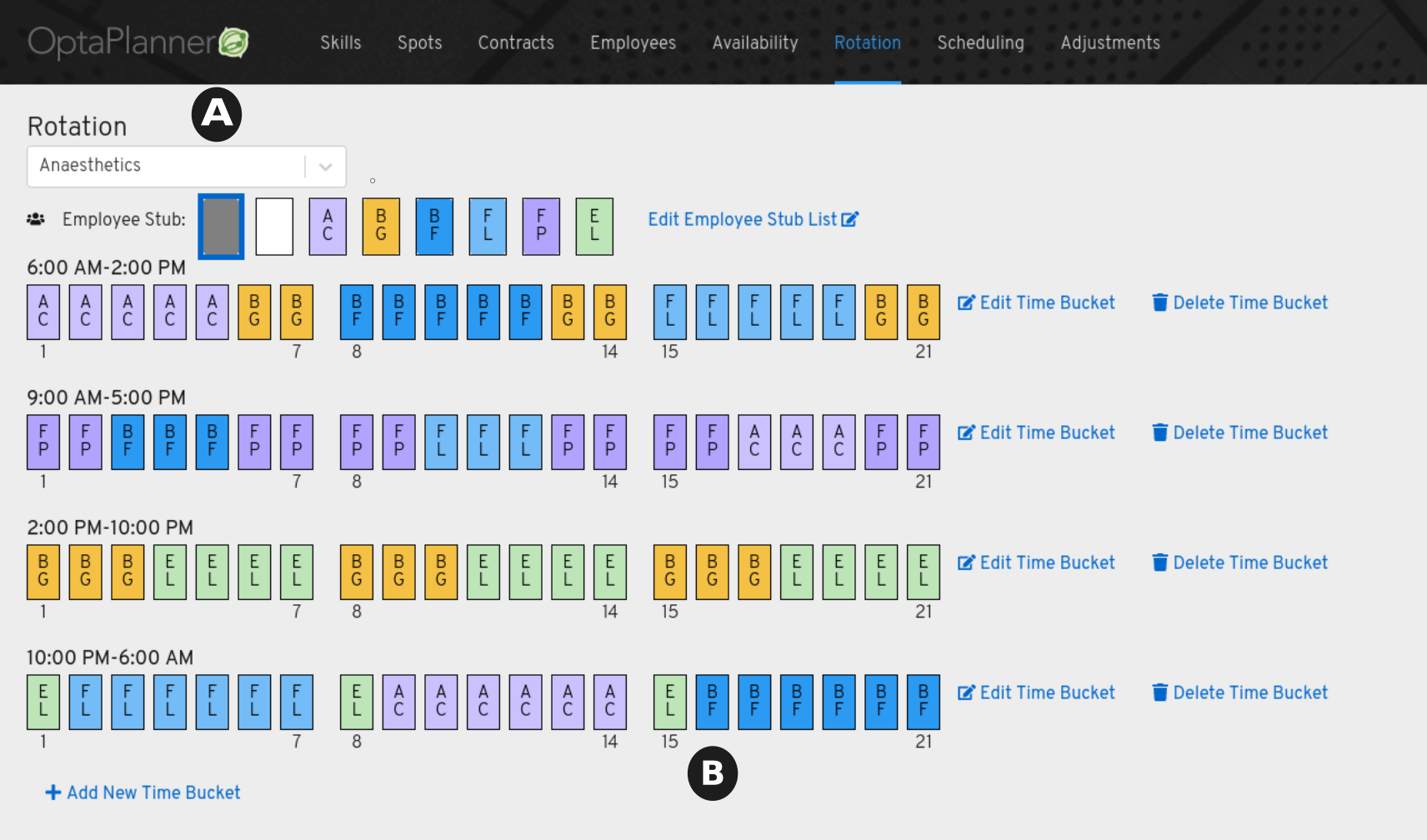
- A time bucket describes a time slot (for example, 9:00 a.m. to 5:00 p.m.) for a particular spot or location (A) (for example, Anaesthetics), over two or more days, and any skills that are required (for example, firearm training).
- A seat (B) is an employee assignment for a particular day in a specific time bucket.
- An employee stub is an icon that represents an employee that is available to be assigned to a time bucket. Employee stubs are listed in the Employee Stub List.
For more information about the rotation pattern, see Section 20.2, “The rotation pattern”.
Procedure
- Click the Rotation tab to view and edit the rotation pattern.
- Select a spot from the Rotation menu.
- Click Add New Time Bucket. The Creating Working Time Bucket dialog is displayed.
- Specify a start and end time, select any additional required skills, select the days for this time bucket, and click Save. The unassigned seats for that time bucket appears on the Rotation page organized by time ranges.
- To create an employee stub list so that you can add employees to the rotation, click Edit Employee Stub List.
- In the Edit Employee Stub List dialog, click Add Employee and select an employee from the list.
- Add all of the employees required for this stub list and click Save. The employees appear above the time buckets on the Rotation page.
- Click an employee icon to select an employee from the employee stub list.
Click and drag the mouse over the seats of a time bucket to assign the selected employee to those seats. The seat is populated with the employee icon.
NoteA time bucket can only have one employee assigned to it for each day. To add multiple employees to the same time bucket, copy the time bucket and change the employee name as required.
- To provision the schedule, click Scheduling and select the spot that you created the rotation for.
- Click Provision and specify the date range.
- Deselect the spots that you do not want to include in this schedule.
- Click the arrow next to the selected spot and deselect any time buckets that you do not want to use in your schedule.
- Click Provision Shifts. The calendar is populated with shifts generated from the time buckets.
- To modify a shift, click a generated shift on the calendar.
Part V. Using Red Hat Business Optimizer with Spring Boot
This guide walks you through the process of creating a Spring Boot application with Red Hat Business Optimizer’s constraint solving artificial intelligence (AI). You will build a REST application that optimizes a school timetable for students and teachers.
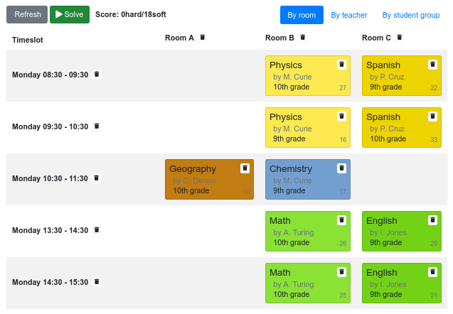
Your service will assign Lesson instances to Timeslot and Room instances automatically by using AI to adhere to the following hard and soft scheduling constraints:
- A room can have at most one lesson at the same time.
- A teacher can teach at most one lesson at the same time.
- A student can attend at most one lesson at the same time.
- A teacher prefers to teach in a single room.
- A teacher prefers to teach sequential lessons and dislikes gaps between lessons.
Mathematically speaking, school timetabling is an NP-hard problem. That means it is difficult to scale. Simply iterating through all possible combinations with brute force would take millions of years for a non-trivial dataset, even on a supercomputer. Fortunately, AI constraint solvers such as Red Hat Business Optimizer have advanced algorithms that deliver a near-optimal solution in a reasonable amount of time. What is considered to be a reasonable amount of time is subjective and depends on the goals of your problem.
Prerequisites
- OpenJDK 8 or later is installed. Red Hat build of Open JDK is available from the Software Downloads page in the Red Hat Customer Portal (login required).
- Apache Maven 3.2 or higher is installed. Maven is available from the Apache Maven Project website.
- An IDE, such as IntelliJ IDEA, VSCode, Eclipse, or NetBeans is available.
Chapter 21. Downloading and building the school timetable reference implementation
If you want to see a completed example of the school timetable project for Red Hat Business Optimizer with Spring Boot product, download the starter application from the Red Hat Customer Portal.
Procedure
Navigate to the Software Downloads page in the Red Hat Customer Portal (login required), and select the product and version from the drop-down options:
- Product: Red Hat Process Automation Manager
- Version: 7.10
-
Download Red Hat Process Automation Manager 7.10 Reference Implementations (
rhpam-7.10.0-reference-implementation.zip). -
Download Red Hat Process Automation Manager 7.10 Maven Repository (
rhpam-7.10.0-maven-repository.zip). -
Extract the
rhpam-7.10.0-maven-repository.zipfile. -
Copy the contents of the
rhpam-7.10.0-maven-repository/maven-repositorysubdirectory into the~/.m2/repositorydirectory. -
Extract the
rhpam-7.10.0-reference-implementation.zipfile. This archive contains reference implementation ZIP files. -
Extract the
rhpam-7.10.0-reference-implementation/rhpam-7.10.0-optaplanner-spring-boot-school-timetabling.zipfile. -
Navigate to the
optaplanner-spring-boot-school-timetabling-7.48.0.Final-redhat-00004directory. Enter the following command to build the Spring Boot school timetabling project:
mvn clean install -DskipTests
To build the Spring Boot school timetabling project, enter the following command:
mvn spring-boot:run -DskipTests
To view the project, enter the following URL in a web browser:
http://localhost:8080/
Chapter 22. Model the domain objects
The goal of the Red Hat Business Optimizer timetable project is to assign each lesson to a time slot and a room. To do this, add three classes, Timeslot, Lesson, and Room, as shown in the following diagram:
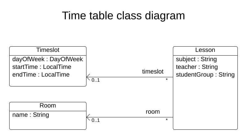
Timeslot
The Timeslot class represents a time interval when lessons are taught, for example, Monday 10:30 - 11:30 or Tuesday 13:30 - 14:30. In this example, all time slots have the same duration and there are no time slots during lunch or other breaks.
A time slot has no date because a high school schedule just repeats every week. There is no need for continuous planning. A Timeslot is called a problem fact because no Timeslot instances change during solving. Such classes do not require any Red Hat Business Optimizer specific annotations.
Room
The Room class represents a location where lessons are taught, for example, Room A or Room B. In this example, all rooms are without capacity limits and they can accommodate all lessons.
Room instances do not change during solving so Room is also a problem fact.
Lesson
During a lesson, represented by the Lesson class, a teacher teaches a subject to a group of students, for example, Math by A.Turing for 9th grade or Chemistry by M.Curie for 10th grade. If a subject is taught multiple times each week by the same teacher to the same student group, there are multiple Lesson instances that are only distinguishable by id. For example, the 9th grade has six math lessons a week.
During solving, Red Hat Business Optimizer changes the timeslot and room fields of the Lesson class to assign each lesson to a time slot and a room. Because Red Hat Business Optimizer changes these fields, Lesson is a planning entity:
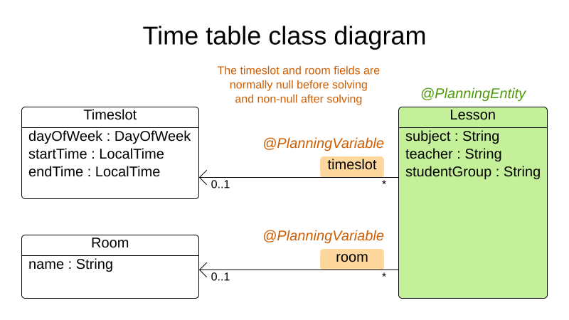
Most of the fields in the previous diagram contain input data, except for the orange fields. A lesson’s timeslot and room fields are unassigned (null) in the input data and assigned (not null) in the output data. Red Hat Business Optimizer changes these fields during solving. Such fields are called planning variables. In order for Red Hat Business Optimizer to recognize them, both the timeslot and room fields require an @PlanningVariable annotation. Their containing class, Lesson, requires an @PlanningEntity annotation.
Procedure
Create the
src/main/java/com/example/domain/Timeslot.javaclass:package com.example.domain; import java.time.DayOfWeek; import java.time.LocalTime; public class Timeslot { private DayOfWeek dayOfWeek; private LocalTime startTime; private LocalTime endTime; private Timeslot() { } public Timeslot(DayOfWeek dayOfWeek, LocalTime startTime, LocalTime endTime) { this.dayOfWeek = dayOfWeek; this.startTime = startTime; this.endTime = endTime; } @Override public String toString() { return dayOfWeek + " " + startTime.toString(); } // ******************************** // Getters and setters // ******************************** public DayOfWeek getDayOfWeek() { return dayOfWeek; } public LocalTime getStartTime() { return startTime; } public LocalTime getEndTime() { return endTime; } }Notice the
toString()method keeps the output short so it is easier to read Red Hat Business Optimizer’sDEBUGorTRACElog, as shown later.Create the
src/main/java/com/example/domain/Room.javaclass:package com.example.domain; public class Room { private String name; private Room() { } public Room(String name) { this.name = name; } @Override public String toString() { return name; } // ******************************** // Getters and setters // ******************************** public String getName() { return name; } }Create the
src/main/java/com/example/domain/Lesson.javaclass:package com.example.domain; import org.optaplanner.core.api.domain.entity.PlanningEntity; import org.optaplanner.core.api.domain.variable.PlanningVariable; @PlanningEntity public class Lesson { private Long id; private String subject; private String teacher; private String studentGroup; @PlanningVariable(valueRangeProviderRefs = "timeslotRange") private Timeslot timeslot; @PlanningVariable(valueRangeProviderRefs = "roomRange") private Room room; private Lesson() { } public Lesson(Long id, String subject, String teacher, String studentGroup) { this.id = id; this.subject = subject; this.teacher = teacher; this.studentGroup = studentGroup; } @Override public String toString() { return subject + "(" + id + ")"; } // ******************************** // Getters and setters // ******************************** public Long getId() { return id; } public String getSubject() { return subject; } public String getTeacher() { return teacher; } public String getStudentGroup() { return studentGroup; } public Timeslot getTimeslot() { return timeslot; } public void setTimeslot(Timeslot timeslot) { this.timeslot = timeslot; } public Room getRoom() { return room; } public void setRoom(Room room) { this.room = room; } }The
Lessonclass has an@PlanningEntityannotation, so Red Hat Business Optimizer knows that this class changes during solving because it contains one or more planning variables.The
timeslotfield has an@PlanningVariableannotation, so Red Hat Business Optimizer knows that it can change its value. In order to find potentialTimeslotinstances to assign to this field, Red Hat Business Optimizer uses thevalueRangeProviderRefsproperty to connect to a value range provider that provides aList<Timeslot>to pick from. See Chapter 24, Gather the domain objects in a planning solution for information about value range providers.The
roomfield also has an@PlanningVariableannotation for the same reasons.
Chapter 23. Define the constraints and calculate the score
When solving a problem, a score represents the quality of a given solution. The higher the score the better. Red Hat Business Optimizer looks for the best solution, which is the solution with the highest score found in the available time. It might be the optimal solution.
Because the timetable example use case has hard and soft constraints, use the HardSoftScore class to represent the score:
- Hard constraints must not be broken. For example: A room can have at most one lesson at the same time.
- Soft constraints should not be broken. For example: A teacher prefers to teach in a single room.
Hard constraints are weighted against other hard constraints. Soft constraints are weighted against other soft constraints. Hard constraints always outweigh soft constraints, regardless of their respective weights.
To calculate the score, you could implement an EasyScoreCalculator class:
public class TimeTableEasyScoreCalculator implements EasyScoreCalculator<TimeTable> {

    @Override
    public HardSoftScore calculateScore(TimeTable timeTable) {
        List<Lesson> lessonList = timeTable.getLessonList();
        int hardScore = 0;
        for (Lesson a : lessonList) {
            for (Lesson b : lessonList) {
                if (a.getTimeslot() != null && a.getTimeslot().equals(b.getTimeslot())
                        && a.getId() < b.getId()) {
                    // A room can accommodate at most one lesson at the same time.
                    if (a.getRoom() != null && a.getRoom().equals(b.getRoom())) {
                        hardScore--;
                    }
                    // A teacher can teach at most one lesson at the same time.
                    if (a.getTeacher().equals(b.getTeacher())) {
                        hardScore--;
                    }
                    // A student can attend at most one lesson at the same time.
                    if (a.getStudentGroup().equals(b.getStudentGroup())) {
                        hardScore--;
                    }
                }
            }
        }
        int softScore = 0;
        // Soft constraints are only implemented in the "complete" implementation
        return HardSoftScore.of(hardScore, softScore);
    }

}
Unfortunately, this solution does not scale well because it is non-incremental: every time a lesson is assigned to a different time slot or room, all lessons are re-evaluated to calculate the new score.
A better solution is to create a src/main/java/com/example/solver/TimeTableConstraintProvider.java class to perform incremental score calculation. This class uses Red Hat Business Optimizer’s ConstraintStream API which is inspired by Java 8 Streams and SQL. The ConstraintProvider scales an order of magnitude better than the EasyScoreCalculator: O(n) instead of O(n²).
Procedure
Create the following src/main/java/com/example/solver/TimeTableConstraintProvider.java class:
package com.example.solver;

import com.example.domain.Lesson;
import org.optaplanner.core.api.score.buildin.hardsoft.HardSoftScore;
import org.optaplanner.core.api.score.stream.Constraint;
import org.optaplanner.core.api.score.stream.ConstraintFactory;
import org.optaplanner.core.api.score.stream.ConstraintProvider;
import org.optaplanner.core.api.score.stream.Joiners;

public class TimeTableConstraintProvider implements ConstraintProvider {

    @Override
    public Constraint[] defineConstraints(ConstraintFactory constraintFactory) {
        return new Constraint[] {
                // Hard constraints
                roomConflict(constraintFactory),
                teacherConflict(constraintFactory),
                studentGroupConflict(constraintFactory),
                // Soft constraints are only implemented in the "complete" implementation
        };
    }

    private Constraint roomConflict(ConstraintFactory constraintFactory) {
        // A room can accommodate at most one lesson at the same time.

        // Select a lesson ...
        return constraintFactory.from(Lesson.class)
                // ... and pair it with another lesson ...
                .join(Lesson.class,
                        // ... in the same timeslot ...
                        Joiners.equal(Lesson::getTimeslot),
                        // ... in the same room ...
                        Joiners.equal(Lesson::getRoom),
                        // ... and the pair is unique (different id, no reverse pairs)
                        Joiners.lessThan(Lesson::getId))
                // then penalize each pair with a hard weight.
                .penalize("Room conflict", HardSoftScore.ONE_HARD);
    }

    private Constraint teacherConflict(ConstraintFactory constraintFactory) {
        // A teacher can teach at most one lesson at the same time.
        return constraintFactory.from(Lesson.class)
                .join(Lesson.class,
                        Joiners.equal(Lesson::getTimeslot),
                        Joiners.equal(Lesson::getTeacher),
                        Joiners.lessThan(Lesson::getId))
                .penalize("Teacher conflict", HardSoftScore.ONE_HARD);
    }

    private Constraint studentGroupConflict(ConstraintFactory constraintFactory) {
        // A student can attend at most one lesson at the same time.
        return constraintFactory.from(Lesson.class)
                .join(Lesson.class,
                        Joiners.equal(Lesson::getTimeslot),
                        Joiners.equal(Lesson::getStudentGroup),
                        Joiners.lessThan(Lesson::getId))
                .penalize("Student group conflict", HardSoftScore.ONE_HARD);
    }

}
Chapter 24. Gather the domain objects in a planning solution
A TimeTable instance wraps all Timeslot, Room, and Lesson instances of a single dataset. Furthermore, because it contains all lessons, each with a specific planning variable state, it is a planning solution and it has a score:
-
If lessons are still unassigned, then it is an uninitialized solution, for example, a solution with the score
-4init/0hard/0soft. -
If it breaks hard constraints, then it is an infeasible solution, for example, a solution with the score
-2hard/-3soft. -
If it adheres to all hard constraints, then it is a feasible solution, for example, a solution with the score
0hard/-7soft.
The TimeTable class has an @PlanningSolution annotation, so Red Hat Business Optimizer knows that this class contains all of the input and output data.
Specifically, this class is the input of the problem:
A
timeslotListfield with all time slots- This is a list of problem facts, because they do not change during solving.
A
roomListfield with all rooms- This is a list of problem facts, because they do not change during solving.
A
lessonListfield with all lessons- This is a list of planning entities because they change during solving.
Of each
Lesson:-
The values of the
timeslotandroomfields are typically stillnull, so unassigned. They are planning variables. -
The other fields, such as
subject,teacherandstudentGroup, are filled in. These fields are problem properties.
-
The values of the
However, this class is also the output of the solution:
-
A
lessonListfield for which eachLessoninstance has non-nulltimeslotandroomfields after solving -
A
scorefield that represents the quality of the output solution, for example,0hard/-5soft
Procedure
Create the src/main/java/com/example/domain/TimeTable.java class:
package com.example.domain;

import java.util.List;

import org.optaplanner.core.api.domain.solution.PlanningEntityCollectionProperty;
import org.optaplanner.core.api.domain.solution.PlanningScore;
import org.optaplanner.core.api.domain.solution.PlanningSolution;
import org.optaplanner.core.api.domain.solution.drools.ProblemFactCollectionProperty;
import org.optaplanner.core.api.domain.valuerange.ValueRangeProvider;
import org.optaplanner.core.api.score.buildin.hardsoft.HardSoftScore;

@PlanningSolution
public class TimeTable {

    @ValueRangeProvider(id = "timeslotRange")
    @ProblemFactCollectionProperty
    private List<Timeslot> timeslotList;

    @ValueRangeProvider(id = "roomRange")
    @ProblemFactCollectionProperty
    private List<Room> roomList;

    @PlanningEntityCollectionProperty
    private List<Lesson> lessonList;

    @PlanningScore
    private HardSoftScore score;

    private TimeTable() {
    }

    public TimeTable(List<Timeslot> timeslotList, List<Room> roomList,
            List<Lesson> lessonList) {
        this.timeslotList = timeslotList;
        this.roomList = roomList;
        this.lessonList = lessonList;
    }

    // ********************************
    // Getters and setters
    // ********************************

    public List<Timeslot> getTimeslotList() {
        return timeslotList;
    }

    public List<Room> getRoomList() {
        return roomList;
    }

    public List<Lesson> getLessonList() {
        return lessonList;
    }

    public HardSoftScore getScore() {
        return score;
    }

}
The value range providers
The timeslotList field is a value range provider. It holds the Timeslot instances which Red Hat Business Optimizer can pick from to assign to the timeslot field of Lesson instances. The timeslotList field has an @ValueRangeProvider annotation to connect those two, by matching the id with the valueRangeProviderRefs of the @PlanningVariable in the Lesson.
Following the same logic, the roomList field also has an @ValueRangeProvider annotation.
The problem fact and planning entity properties
Furthermore, Red Hat Business Optimizer needs to know which Lesson instances it can change as well as how to retrieve the Timeslot and Room instances used for score calculation by your TimeTableConstraintProvider.
The timeslotList and roomList fields have an @ProblemFactCollectionProperty annotation, so your TimeTableConstraintProvider can select from those instances.
The lessonList has an @PlanningEntityCollectionProperty annotation, so Red Hat Business Optimizer can change them during solving and your TimeTableConstraintProvider can select from those too.
Chapter 25. Create the Timetable service
Now you are ready to put everything together and create a REST service. But solving planning problems on REST threads causes HTTP timeout issues. Therefore, the Spring Boot starter injects a SolverManager, which runs solvers in a separate thread pool and can solve multiple datasets in parallel.
Procedure
Create the src/main/java/com/example/solver/TimeTableController.java class:
package com.example.solver;

import java.util.UUID;
import java.util.concurrent.ExecutionException;

import com.example.domain.TimeTable;
import org.optaplanner.core.api.solver.SolverJob;
import org.optaplanner.core.api.solver.SolverManager;
import org.springframework.beans.factory.annotation.Autowired;
import org.springframework.web.bind.annotation.PostMapping;
import org.springframework.web.bind.annotation.RequestBody;
import org.springframework.web.bind.annotation.RequestMapping;
import org.springframework.web.bind.annotation.RestController;

@RestController
@RequestMapping("/timeTable")
public class TimeTableController {

    @Autowired
    private SolverManager<TimeTable, UUID> solverManager;

    @PostMapping("/solve")
    public TimeTable solve(@RequestBody TimeTable problem) {
        UUID problemId = UUID.randomUUID();
        // Submit the problem to start solving
        SolverJob<TimeTable, UUID> solverJob = solverManager.solve(problemId, problem);
        TimeTable solution;
        try {
            // Wait until the solving ends
            solution = solverJob.getFinalBestSolution();
        } catch (InterruptedException | ExecutionException e) {
            throw new IllegalStateException("Solving failed.", e);
        }
        return solution;
    }

}
In this example, the initial implementation waits for the solver to finish, which can still cause an HTTP timeout. The complete implementation avoids HTTP timeouts much more elegantly.
Chapter 26. Set the solver termination time
If your planning application does not have a termination setting or a termination event, it theoretically runs forever and in reality eventually causes an HTTP timeout error. To prevent this from occurring, use the optaplanner.solver.termination.spent-limit parameter to specify the length of time after which the application terminates. In most applications, set the time to at least five minutes (5m). However, in the Timetable example, limit the solving time to five second, which is short enough to avoid the HTTP timeout.
Procedure
Create the src/main/resources/application.properties file with the following content:
optaplanner.solver.termination.spent-limit=5s
Chapter 27. Make the application executable
After you complete the Red Hat Business Optimizer Spring Boot timetable project, package everything into a single executable JAR file driven by a standard Java main() method.
Prerequisites
- You have a completed Red Hat Business Optimizer Spring Boot timetable project.
Procedure
Create the
TimeTableSpringBootApp.javaclass with the following content:package com.example; import org.springframework.boot.SpringApplication; import org.springframework.boot.autoconfigure.SpringBootApplication; @SpringBootApplication public class TimeTableSpringBootApp { public static void main(String[] args) { SpringApplication.run(TimeTableSpringBootApp.class, args); } }-
Replace the
src/main/java/com/example/DemoApplication.javaclass created by Spring Initializr with theTimeTableSpringBootApp.javaclass. -
Run the
TimeTableSpringBootApp.javaclass as the main class of a regular Java application.
27.1. Try the timetable application
After you start the Red Hat Business Optimizer Spring Boot timetable application, you can test the REST service with any REST client that you want. This example uses the Linux curl command to send a POST request.
Prerequisites
- The Red Hat Business Optimizer Spring Boot timetable application is running.
Procedure
Enter the following command:
$ curl -i -X POST http://localhost:8080/timeTable/solve -H "Content-Type:application/json" -d '{"timeslotList":[{"dayOfWeek":"MONDAY","startTime":"08:30:00","endTime":"09:30:00"},{"dayOfWeek":"MONDAY","startTime":"09:30:00","endTime":"10:30:00"}],"roomList":[{"name":"Room A"},{"name":"Room B"}],"lessonList":[{"id":1,"subject":"Math","teacher":"A. Turing","studentGroup":"9th grade"},{"id":2,"subject":"Chemistry","teacher":"M. Curie","studentGroup":"9th grade"},{"id":3,"subject":"French","teacher":"M. Curie","studentGroup":"10th grade"},{"id":4,"subject":"History","teacher":"I. Jones","studentGroup":"10th grade"}]}'
After about five seconds, the termination spent time defined in application.properties, the service returns an output similar to the following example:
HTTP/1.1 200
Content-Type: application/json
...

{"timeslotList":...,"roomList":...,"lessonList":[{"id":1,"subject":"Math","teacher":"A. Turing","studentGroup":"9th grade","timeslot":{"dayOfWeek":"MONDAY","startTime":"08:30:00","endTime":"09:30:00"},"room":{"name":"Room A"}},{"id":2,"subject":"Chemistry","teacher":"M. Curie","studentGroup":"9th grade","timeslot":{"dayOfWeek":"MONDAY","startTime":"09:30:00","endTime":"10:30:00"},"room":{"name":"Room A"}},{"id":3,"subject":"French","teacher":"M. Curie","studentGroup":"10th grade","timeslot":{"dayOfWeek":"MONDAY","startTime":"08:30:00","endTime":"09:30:00"},"room":{"name":"Room B"}},{"id":4,"subject":"History","teacher":"I. Jones","studentGroup":"10th grade","timeslot":{"dayOfWeek":"MONDAY","startTime":"09:30:00","endTime":"10:30:00"},"room":{"name":"Room B"}}],"score":"0hard/0soft"}
Notice that the application assigned all four lessons to one of the two time slots and one of the two rooms. Also notice that it conforms to all hard constraints. For example, M. Curie’s two lessons are in different time slots.
On the server side, the info log shows what Red Hat Business Optimizer did in those five seconds:
... Solving started: time spent (33), best score (-8init/0hard/0soft), environment mode (REPRODUCIBLE), random (JDK with seed 0).
... Construction Heuristic phase (0) ended: time spent (73), best score (0hard/0soft), score calculation speed (459/sec), step total (4).
... Local Search phase (1) ended: time spent (5000), best score (0hard/0soft), score calculation speed (28949/sec), step total (28398).
... Solving ended: time spent (5000), best score (0hard/0soft), score calculation speed (28524/sec), phase total (2), environment mode (REPRODUCIBLE).
27.2. Test the application
A good application includes test coverage. This example tests the Timetable Red Hat Business Optimizer Spring Boot application. It uses a JUnit test to generate a test dataset and send it to the TimeTableController to solve.
Procedure
Create the src/test/java/com/example/solver/TimeTableControllerTest.java class with the following content:
package com.example.solver;

import java.time.DayOfWeek;
import java.time.LocalTime;
import java.util.ArrayList;
import java.util.List;

import com.example.domain.Lesson;
import com.example.domain.Room;
import com.example.domain.TimeTable;
import com.example.domain.Timeslot;
import org.junit.jupiter.api.Test;
import org.junit.jupiter.api.Timeout;
import org.springframework.beans.factory.annotation.Autowired;
import org.springframework.boot.test.context.SpringBootTest;

import static org.junit.jupiter.api.Assertions.assertFalse;
import static org.junit.jupiter.api.Assertions.assertNotNull;
import static org.junit.jupiter.api.Assertions.assertTrue;

@SpringBootTest(properties = {
        "optaplanner.solver.termination.spent-limit=1h", // Effectively disable this termination in favor of the best-score-limit
        "optaplanner.solver.termination.best-score-limit=0hard/*soft"})
public class TimeTableControllerTest {

    @Autowired
    private TimeTableController timeTableController;

    @Test
    @Timeout(600_000)
    public void solve() {
        TimeTable problem = generateProblem();
        TimeTable solution = timeTableController.solve(problem);
        assertFalse(solution.getLessonList().isEmpty());
        for (Lesson lesson : solution.getLessonList()) {
            assertNotNull(lesson.getTimeslot());
            assertNotNull(lesson.getRoom());
        }
        assertTrue(solution.getScore().isFeasible());
    }

    private TimeTable generateProblem() {
        List<Timeslot> timeslotList = new ArrayList<>();
        timeslotList.add(new Timeslot(DayOfWeek.MONDAY, LocalTime.of(8, 30), LocalTime.of(9, 30)));
        timeslotList.add(new Timeslot(DayOfWeek.MONDAY, LocalTime.of(9, 30), LocalTime.of(10, 30)));
        timeslotList.add(new Timeslot(DayOfWeek.MONDAY, LocalTime.of(10, 30), LocalTime.of(11, 30)));
        timeslotList.add(new Timeslot(DayOfWeek.MONDAY, LocalTime.of(13, 30), LocalTime.of(14, 30)));
        timeslotList.add(new Timeslot(DayOfWeek.MONDAY, LocalTime.of(14, 30), LocalTime.of(15, 30)));

        List<Room> roomList = new ArrayList<>();
        roomList.add(new Room("Room A"));
        roomList.add(new Room("Room B"));
        roomList.add(new Room("Room C"));

        List<Lesson> lessonList = new ArrayList<>();
        lessonList.add(new Lesson(101L, "Math", "B. May", "9th grade"));
        lessonList.add(new Lesson(102L, "Physics", "M. Curie", "9th grade"));
        lessonList.add(new Lesson(103L, "Geography", "M. Polo", "9th grade"));
        lessonList.add(new Lesson(104L, "English", "I. Jones", "9th grade"));
        lessonList.add(new Lesson(105L, "Spanish", "P. Cruz", "9th grade"));

        lessonList.add(new Lesson(201L, "Math", "B. May", "10th grade"));
        lessonList.add(new Lesson(202L, "Chemistry", "M. Curie", "10th grade"));
        lessonList.add(new Lesson(203L, "History", "I. Jones", "10th grade"));
        lessonList.add(new Lesson(204L, "English", "P. Cruz", "10th grade"));
        lessonList.add(new Lesson(205L, "French", "M. Curie", "10th grade"));
        return new TimeTable(timeslotList, roomList, lessonList);
    }

}
This test verifies that after solving, all lessons are assigned to a time slot and a room. It also verifies that it found a feasible solution (no hard constraints broken).
Normally, the solver finds a feasible solution in less than 200 milliseconds. Notice how the @SpringBootTest annotation’s properties overwrites the solver termination to terminate as soon as a feasible solution (0hard/*soft) is found. This avoids hard coding a solver time, because the unit test might run on arbitrary hardware. This approach ensures that the test runs long enough to find a feasible solution, even on slow machines. However, it does not run a millisecond longer than it strictly must, even on fast machines.
27.3. Logging
After you complete the Red Hat Business Optimizer Spring Boot timetable application, you can use logging information to help you fine-tune the constraints in the ConstraintProvider. Review the score calculation speed in the info log file to assess the impact of changes to your constraints. Run the application in debug mode to show every step that your application takes or use trace logging to log every step and every move.
Procedure
- Run the timetable application for a fixed amount of time, for example, five minutes.
Review the score calculation speed in the
logfile as shown in the following example:... Solving ended: ..., score calculation speed (29455/sec), ...
-
Change a constraint, run the planning application again for the same amount of time, and review the score calculation speed recorded in the
logfile. Run the application in debug mode to log every step:
-
To run debug mode from the command line, use the
-Dsystem property. To change logging in the
application.propertiesfile, add the following line to that file:logging.level.org.optaplanner=debug
The following example shows output in the
logfile in debug mode:... Solving started: time spent (67), best score (-20init/0hard/0soft), environment mode (REPRODUCIBLE), random (JDK with seed 0). ... CH step (0), time spent (128), score (-18init/0hard/0soft), selected move count (15), picked move ([Math(101) {null -> Room A}, Math(101) {null -> MONDAY 08:30}]). ... CH step (1), time spent (145), score (-16init/0hard/0soft), selected move count (15), picked move ([Physics(102) {null -> Room A}, Physics(102) {null -> MONDAY 09:30}]). ...
-
To run debug mode from the command line, use the
-
Use
tracelogging to show every step and every move per step.
Chapter 28. Add Database and UI integration
After you create the Red Hat Business Optimizer application example with Spring Boot, add database and UI integration.
Prerequisite
- You have created the Red Hat Business Optimizer Spring Boot timetable example.
Procedure
-
Create Java Persistence API (JPA) repositories for
Timeslot,Room, andLesson. For information about creating JPA repositories, see Accessing Data with JPA on the Spring website. - Expose the JPA repositories through REST. For information about exposing the repositories, see Accessing JPA Data with REST on the Spring website.
-
Build a
TimeTableRepositoryfacade to read and write aTimeTablein a single transaction. Adjust the
TimeTableControlleras shown in the following example:package com.example.solver; import com.example.domain.TimeTable; import com.example.persistence.TimeTableRepository; import org.optaplanner.core.api.score.ScoreManager; import org.optaplanner.core.api.solver.SolverManager; import org.optaplanner.core.api.solver.SolverStatus; import org.springframework.beans.factory.annotation.Autowired; import org.springframework.web.bind.annotation.GetMapping; import org.springframework.web.bind.annotation.PostMapping; import org.springframework.web.bind.annotation.RequestMapping; import org.springframework.web.bind.annotation.RestController; @RestController @RequestMapping("/timeTable") public class TimeTableController { @Autowired private TimeTableRepository timeTableRepository; @Autowired private SolverManager<TimeTable, Long> solverManager; @Autowired private ScoreManager<TimeTable> scoreManager; // To try, GET http://localhost:8080/timeTable @GetMapping() public TimeTable getTimeTable() { // Get the solver status before loading the solution // to avoid the race condition that the solver terminates between them SolverStatus solverStatus = getSolverStatus(); TimeTable solution = timeTableRepository.findById(TimeTableRepository.SINGLETON_TIME_TABLE_ID); scoreManager.updateScore(solution); // Sets the score solution.setSolverStatus(solverStatus); return solution; } @PostMapping("/solve") public void solve() { solverManager.solveAndListen(TimeTableRepository.SINGLETON_TIME_TABLE_ID, timeTableRepository::findById, timeTableRepository::save); } public SolverStatus getSolverStatus() { return solverManager.getSolverStatus(TimeTableRepository.SINGLETON_TIME_TABLE_ID); } @PostMapping("/stopSolving") public void stopSolving() { solverManager.terminateEarly(TimeTableRepository.SINGLETON_TIME_TABLE_ID); } }For simplicity, this code handles only one
TimeTableinstance, but it is straightforward to enable multi-tenancy and handle multipleTimeTableinstances of different high schools in parallel.The
getTimeTable()method returns the latest timetable from the database. It uses theScoreManager(which is automatically injected) to calculate the score of that timetable so the UI can show the score.The
solve()method starts a job to solve the current timetable and store the time slot and room assignments in the database. It uses theSolverManager.solveAndListen()method to listen to intermediate best solutions and update the database accordingly. This enables the UI to show progress while the backend is still solving.Now that the
solve()method returns immediately, adjust theTimeTableControllerTestas shown in the following example:package com.example.solver; import com.example.domain.Lesson; import com.example.domain.TimeTable; import org.junit.jupiter.api.Test; import org.junit.jupiter.api.Timeout; import org.optaplanner.core.api.solver.SolverStatus; import org.springframework.beans.factory.annotation.Autowired; import org.springframework.boot.test.context.SpringBootTest; import static org.junit.jupiter.api.Assertions.assertFalse; import static org.junit.jupiter.api.Assertions.assertNotNull; import static org.junit.jupiter.api.Assertions.assertTrue; @SpringBootTest(properties = { "optaplanner.solver.termination.spent-limit=1h", // Effectively disable this termination in favor of the best-score-limit "optaplanner.solver.termination.best-score-limit=0hard/*soft"}) public class TimeTableControllerTest { @Autowired private TimeTableController timeTableController; @Test @Timeout(600_000) public void solveDemoDataUntilFeasible() throws InterruptedException { timeTableController.solve(); TimeTable timeTable = timeTableController.getTimeTable(); while (timeTable.getSolverStatus() != SolverStatus.NOT_SOLVING) { // Quick polling (not a Test Thread Sleep anti-pattern) // Test is still fast on fast machines and doesn't randomly fail on slow machines. Thread.sleep(20L); timeTable = timeTableController.getTimeTable(); } assertFalse(timeTable.getLessonList().isEmpty()); for (Lesson lesson : timeTable.getLessonList()) { assertNotNull(lesson.getTimeslot()); assertNotNull(lesson.getRoom()); } assertTrue(timeTable.getScore().isFeasible()); } }- Poll for the latest solution until the solver finishes solving.
- To visualize the timetable, build an attractive web UI on top of these REST methods.
Appendix A. Versioning information
Documentation last updated on Tuesday, March 8, 2022.
Appendix B. Contact information
Red Hat Process Automation Manager documentation team: brms-docs@redhat.com