
Chapter 10. Federated Planning
At its core, Data Virtualization is a federated, relational query engine. This query engine allows you to treat all of your data sources as one virtual database, and access them through a single SQL query. As a result, instead of focusing on hand-coding joins, you can focus on building your application, and on running other relational operations between data sources.
10.1. Planning Overview
When the query engine receives an incoming SQL query it performs the following operations:
- Parsing — Validates syntax and convert to internal form.
- Resolving — Links all identifiers to metadata and functions to the function library.
- Validating — Validates SQL semantics based on metadata references and type signatures.
- Rewriting — Rewrites SQL to simplify expressions and criteria.
- Logical plan optimization — Converts the rewritten canonical SQL to a logical plan for in-depth optimization. The Data Virtualization optimizer is predominantly rule-based. Based upon the query structure and hints, a certain rule set will be applied. These rules may trigger in turn trigger the execution of more rules. Within several rules, Data Virtualization also takes advantage of costing information. The logical plan optimization steps can be seen by using the `SET SHOWPLAN DEBUG`clause, as described in the Client Development Guide. For sample steps, see Reading a debug plan in Query Planner. For more information about logical plan nodes and rule-based optimization, see Query Planner.
- Processing plan conversion — Converts the logic plan to an executable form where the nodes represent basic processing operations. The final processing plan is displayed as a query plan. For more information, see Query plans.
The logical query plan is a tree of operations that is used to transform data in source tables to the expected result set. In the tree, data flows from the bottom (tables) to the top (output). The primary logical operations are select (select or filter rows based on a criteria), project (project or compute column values), join, source (retrieve data from a table), sort (ORDER BY), duplicate removal (SELECT DISTINCT), group (GROUP BY), and union (UNION).
For example, consider the following query that retrieves all engineering employees born since 1970.
Example query
SELECT e.title, e.lastname FROM Employees AS e JOIN Departments AS d ON e.dept_id = d.dept_id WHERE year(e.birthday) >= 1970 AND d.dept_name = 'Engineering'
Logically, the data from the Employees and Departments tables are retrieved, then joined, then filtered as specified, and finally the output columns are projected. The canonical query plan thus looks like this:
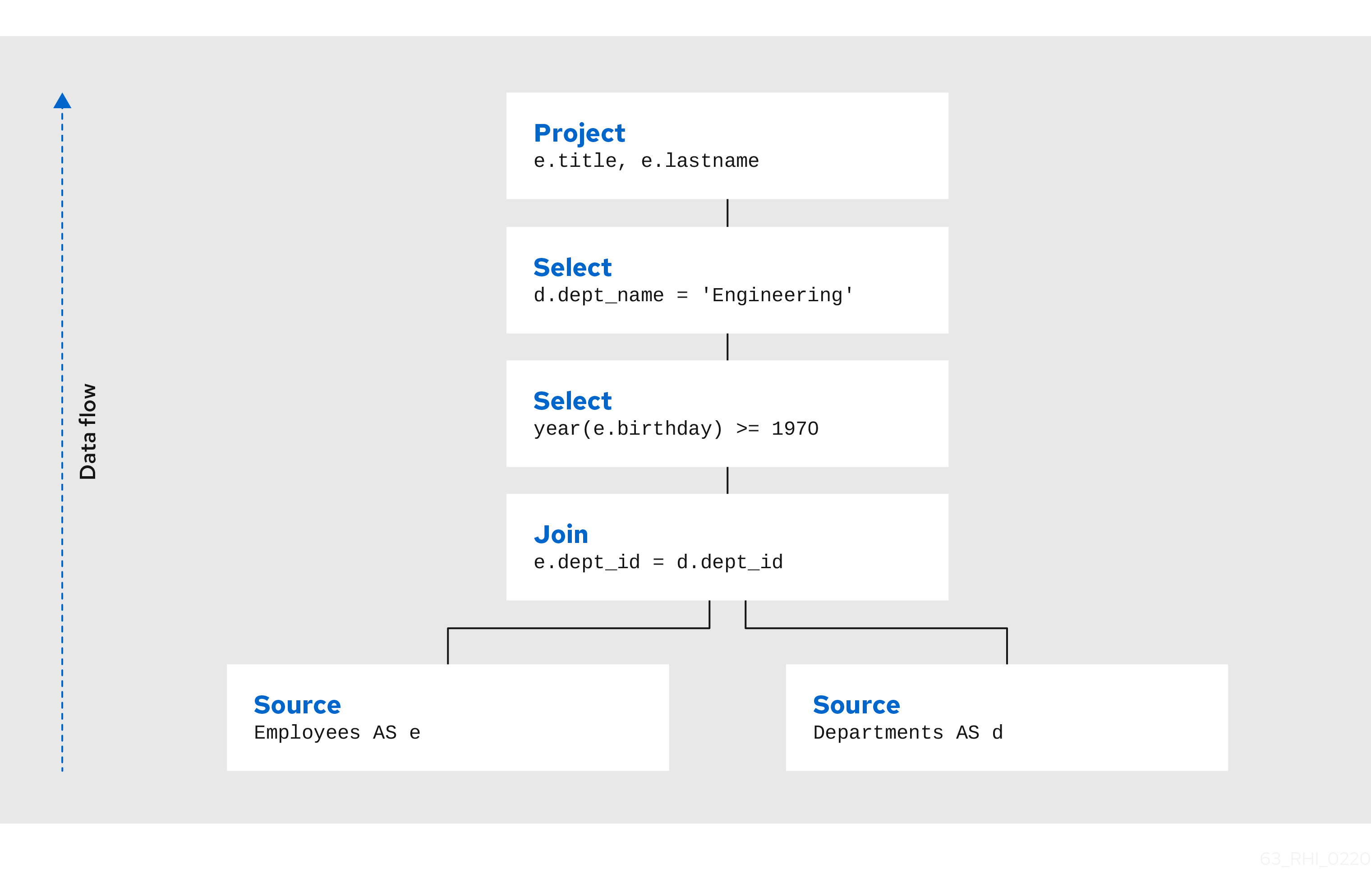
Data flows from the tables at the bottom upwards through the join, through the select, and finally through the project to produce the final results. The data passed between each node is logically a result set with columns and rows.
Of course, this is what happens logically — it is not how the plan is actually executed. Starting from this initial plan, the query planner performs transformations on the query plan tree to produce an equivalent plan that retrieves the same results faster. Both a federated query planner and a relational database planner deal with the same concepts and many of the same plan transformations. In this example, the criteria on the Departments and Employees tables will be pushed down the tree to filter the results as early as possible.
In both cases, the goal is to retrieve the query results in the fastest possible time. However, the relational database planner achieve this primarily by optimizing the access paths in pulling data from storage.
In contrast, a federated query planner is less concerned about storage access, because it is typically pushing that burden to the data source. The most important consideration for a federated query planner is minimizing data transfer.
10.2. Query planner
For each sub-command in the user command an appropriate kind of sub-planner is used (relational, XML, procedure, etc).
Each planner has three primary phases:
- Generate canonical plan
- Optimization
- Plan to process converter — Converts plan data structure into a processing form.
Relational planner
A relational processing plan is created by the optimizer after the logical plan is manipulated by a series of rules. The application of rules is determined both by the query structure and by the rules themselves. The node structure of the debug plan resembles that of the processing plan, but the node types more logically represent SQL operations.
Canonical plan and all nodes
As described in the Planning overview, a SQL statement submitted to the query engine is parsed, resolved, validated, and rewritten before it is converted into a canonical plan form. The canonical plan form most closely resembles the initial SQL structure. A SQL select query has the following possible clauses (all but SELECT are optional): WITH, SELECT, FROM, WHERE, GROUP BY, HAVING, ORDER BY, LIMIT. These clauses are logically executed in the following order:
- WITH (create common table expressions) — Processed by a specialized PROJECT NODE.
- FROM (read and join all data from tables) — Processed by a SOURCE node for each from clause item, or a Join node (if >1 table).
- WHERE (filter rows) — Processed by a SELECT node.
- GROUP BY (group rows into collapsed rows) — Processed by a GROUP node.
- HAVING (filter grouped rows) — Processed by a SELECT node.
- SELECT (evaluate expressions and return only requested rows) — Processed by a PROJECT node and DUP_REMOVE node (for SELECT DISTINCT).
- INTO — Processed by a specialized PROJECT with a SOURCE child.
- ORDER BY (sort rows) — Processed by a SORT node.
- LIMIT (limit result set to a certain range of results) — Processed by a LIMIT node.
For example, a SQL statement such as SELECT max(pm1.g1.e1) FROM pm1.g1 WHERE e2 = 1 creates a logical plan:
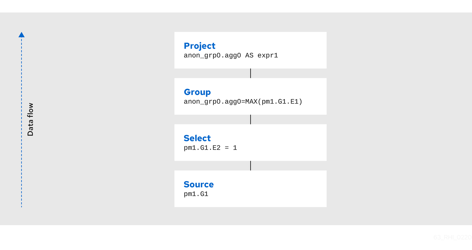
Project(groups=[anon_grp0], props={PROJECT_COLS=[anon_grp0.agg0 AS expr1]})
  Group(groups=[anon_grp0], props={SYMBOL_MAP={anon_grp0.agg0=MAX(pm1.G1.E1)}})
    Select(groups=[pm1.G1], props={SELECT_CRITERIA=pm1.G1.E2 = 1})
      Source(groups=[pm1.G1])
Here the Source corresponds to the FROM clause, the Select corresponds to the WHERE clause, the Group corresponds to the implied grouping to create the max aggregate, and the Project corresponds to the SELECT clause.
The effect of grouping generates what is effectively an inline view, anon_grp0, to handle the projection of values created by the grouping.
Table 10.1. Node Types
| Type Name | Description |
|---|---|
| ACCESS | A source access or plan execution. |
| DUP_REMOVE | Removes duplicate rows |
| JOIN | A join (LEFT OUTER, FULL OUTER, INNER, CROSS, SEMI, and so forth). |
| PROJECT | A projection of tuple values |
| SELECT | A filtering of tuples |
| SORT | An ordering operation, which may be inserted to process other operations such as joins. |
| SOURCE | Any logical source of tuples including an inline view, a source access, XMLTABLE, and so forth. |
| GROUP | A grouping operation. |
| SET_OP | A set operation (UNION/INTERSECT/EXCEPT). |
| NULL | A source of no tuples. |
| TUPLE_LIMIT | Row offset / limit |
Node properties
Each node has a set of applicable properties that are typically shown on the node.
Table 10.2. Access properties
| Property Name | Description |
|---|---|
| ATOMIC_REQUEST | The final form of a source request. |
| MODEL_ID | The metadata object for the target model/schema. |
| PROCEDURE_CRITERIA/PROCEDURE_INPUTS/PROCEDURE_DEFAULTS | Used in planning procedureal relational queries. |
| IS_MULTI_SOURCE | set to true when the node represents a multi-source access. |
| SOURCE_NAME | used to track the multi-source source name. |
| CONFORMED_SOURCES | tracks the set of conformed sources when the conformed extension metadata is used. |
| SUB_PLAN/SUB_PLANS | used in multi-source planning. |
Table 10.3. Set operation properties
| Property Name | Description |
|---|---|
| SET_OPERATION/USE_ALL | defines the set operation(UNION/INTERSECT/EXCEPT) and if all rows or distinct rows are used. |
Table 10.4. Join properties
| Property Name | Description |
|---|---|
| JOIN_CRITERIA | All join predicates. |
| JOIN_TYPE | Type of join (INNER, LEFT OUTER, and so forth). |
| JOIN_STRATEGY | The algorithm to use (nested loop, merge, and so forth). |
| LEFT_EXPRESSIONS | The expressions in equi-join predicates that originate from the left side of the join. |
| RIGHT_EXPRESSIONS | The expressions in equi-join predicates that originate from the right side of the join. |
| DEPENDENT_VALUE_SOURCE | set if a dependent join is used. |
| NON_EQUI_JOIN_CRITERIA | Non-equi join predicates. |
| SORT_LEFT | If the left side needs sorted for join processing. |
| SORT_RIGHT | If the right side needs sorted for join processing. |
| IS_OPTIONAL | If the join is optional. |
| IS_LEFT_DISTINCT | If the left side is distinct with respect to the equi join predicates. |
| IS_RIGHT_DISTINCT | If the right side is distinct with respect to the equi join predicates. |
| IS_SEMI_DEP | If the dependent join represents a semi-join. |
| PRESERVE | If the preserve hint is preserving the join order. |
Table 10.5. Project properties
| Property Name | Description |
|---|---|
| PROJECT_COLS | The expressions projected. |
| INTO_GROUP | The group targeted if this is a select into or insert with a query expression. |
| HAS_WINDOW_FUNCTIONS | True if window functions are used. |
| CONSTRAINT | The constraint that must be met if the values are being projected into a group. |
| UPSERT | If the insert is an upsert. |
Table 10.6. Select properties
| Property Name | Description |
|---|---|
| SELECT_CRITERIA | The filter. |
| IS_HAVING | If the filter is applied after grouping. |
| IS_PHANTOM | True if the node is marked for removal, but temporarily left in the plan. |
| IS_TEMPORARY | Inferred criteria that may not be used in the final plan. |
| IS_COPIED | If the criteria has already been processed by rule copy criteria. |
| IS_PUSHED | If the criteria is pushed as far as possible. |
| IS_DEPENDENT_SET | If the criteria is the filter of a dependent join. |
Table 10.7. Sort properties
| Property Name | Description |
|---|---|
| SORT_ORDER | The order by that defines the sort. |
| UNRELATED_SORT | If the ordering includes a value that is not being projected. |
| IS_DUP_REMOVAL | If the sort should also perform duplicate removal over the entire projection. |
Table 10.8. Source properties
| Property Name | Description |
|---|---|
| SYMBOL_MAP | The mapping from the columns above the source to the projected expressions. Also present on Group nodes. |
| PARTITION_INFO | The partitioning of the union branches. |
| VIRTUAL_COMMAND | If the source represents an view or inline view, the query that defined the view. |
| MAKE_DEP | Hint information. |
| PROCESSOR_PLAN | The processor plan of a non-relational source(typically from the NESTED_COMMAND). |
| NESTED_COMMAND | The non-relational command. |
| TABLE_FUNCTION | The table function (XMLTABLE, OBJECTTABLE, and so forth.) defining the source. |
| CORRELATED_REFERENCES | The correlated references for the nodes below the source. |
| MAKE_NOT_DEP | If make not dep is set. |
| INLINE_VIEW | If the source node represents an inline view. |
| NO_UNNEST | If the no_unnest hint is set. |
| MAKE_IND | If the make ind hint is set. |
| SOURCE_HINT | The source hint. See Federated optimizations. |
| ACCESS_PATTERNS | Access patterns yet to be satisfied. |
| ACCESS_PATTERN_USED | Satisfied access patterns. |
| REQUIRED_ACCESS_PATTERN_GROUPS | Groups needed to satisfy the access patterns. Used in join planning. |
Many source properties also become present on associated access nodes.
Table 10.9. Group properties
| Property Name | Description |
|---|---|
| GROUP_COLS | The grouping columns. |
| ROLLUP | If the grouping includes a rollup. |
Table 10.10. Tuple limit properties
| Property Name | Description |
|---|---|
| MAX_TUPLE_LIMIT | Expression that evaluates to the max number of tuples generated. |
| OFFSET_TUPLE_COUNT | Expression that evaluates to the tuple offset of the starting tuple. |
| IS_IMPLICIT_LIMIT | If the limit is created by the rewriter as part of a subquery optimization. |
| IS_NON_STRICT | If the unordered limit should not be enforced strictly. |
Table 10.11. General and costing properties
| Property Name | Description |
|---|---|
| OUTPUT_COLS | The output columns for the node. Is typically set after rule assign output elements. |
| EST_SET_SIZE | Represents the estimated set size this node would produce for a sibling node as the independent node in a dependent join scenario. |
| EST_DEP_CARDINALITY | Value that represents the estimated cardinality (amount of rows) produced by this node as the dependent node in a dependent join scenario. |
| EST_DEP_JOIN_COST | Value that represents the estimated cost of a dependent join (the join strategy for this could be Nested Loop or Merge). |
| EST_JOIN_COST | Value that represents the estimated cost of a merge join (the join strategy for this could be Nested Loop or Merge). |
| EST_CARDINALITY | Represents the estimated cardinality (amount of rows) produced by this node. |
| EST_COL_STATS | Column statistics including number of null values, distinct value count, and so forth. |
| EST_SELECTIVITY | Represents the selectivity of a criteria node. |
Rules
Relational optimization is based upon rule execution that evolves the initial plan into the execution plan. There are a set of pre-defined rules that are dynamically assembled into a rule stack for every query. The rule stack is assembled based on the contents of the user’s query and the views/procedures accessed. For example, if there are no view layers, then rule Merge Virtual, which merges view layers together, is not needed and will not be added to the stack. This allows the rule stack to reflect the complexity of the query.
Logically the plan node data structure represents a tree of nodes where the source data comes up from the leaf nodes (typically Access nodes in the final plan), flows up through the tree and produces the user’s results out the top. The nodes in the plan structure can have bidirectional links, dynamic properties, and allow any number of child nodes. Processing plans in contrast typically have fixed properties.
Plan rule manipulate the plan tree, fire other rules, and drive the optimization process. Each rule is designed to perform a narrow set of tasks. Some rules can be run multiple times. Some rules require a specific set of precursors to run properly.
- Access Pattern Validation — Ensures that all access patterns have been satisfied.
- Apply Security — Applies row and column level security.
- Assign Output Symbol — This rule walks top down through every node and calculates the output columns for each node. Columns that are not needed are dropped at every node, which is known as projection minimization. This is done by keeping track of both the columns needed to feed the parent node and also keeping track of columns that are "created" at a certain node.
- Calculate Cost — Adds costing information to the plan
Choose Dependent — This rule looks at each join node and determines whether the join should be made dependent and in which direction. Cardinality, the number of distinct values, and primary key information are used in several formulas to determine whether a dependent join is likely to be worthwhile. The dependent join differs in performance ideally because a fewer number of values will be returned from the dependent side.
Also, we must consider the number of values passed from independent to dependent side. If that set is larger than the maximum number of values in an IN criteria on the dependent side, then we must break the query into a set of queries and combine their results. Executing each query in the connector has some overhead and that is taken into account. Without costing information a lot of common cases where the only criteria specified is on a non-unique (but strongly limiting) field are missed.
A join is eligible to be dependent if:
-
There is at least one equi-join criterion, for example,
tablea.col = tableb.col - The join is not a full outer join and the dependent side of the join is on the inner side of the join.
-
There is at least one equi-join criterion, for example,
The join will be made dependent if one of the following conditions, listed in precedence order, holds:
- There is an unsatisfied access pattern that can be satisfied with the dependent join criteria.
- The potential dependent side of the join is marked with an option makedep.
- (4.3.2) if costing was enabled, the estimated cost for the dependent join (5.0+ possibly in each direction in the case of inner joins) is computed and compared to not performing the dependent join. If the costs were all determined (which requires all relevant table cardinality, column ndv, and possibly nnv values to be populated) the lowest is chosen.
- If key metadata information indicates that the potential dependent side is not "small" and the other side is "not small" or (5.0.1) the potential dependent side is the inner side of a left outer join.
Dependent join is the key optimization we use to efficiently process multi-source joins. Instead of reading all of source A and all of source B and joining them on A.x = B.x, we read all of A, and then build a set of A.x that are passed as a criteria when querying B. In cases where A is small and B is large, this can drastically reduce the data retrieved from B, thus greatly speeding the overall query.
- Choose Join Strategy — Choose the join strategy based upon the cost and attributes of the join.
- Clean Criteria — Removes phantom criteria.
- Collapse Source — Takes all of the nodes below an access node and creates a SQL query representation.
- Copy Criteria — This rule copies criteria over an equality criteria that is present in the criteria of a join. Since the equality defines an equivalence, this is a valid way to create a new criteria that may limit results on the other side of the join (especially in the case of a multi-source join).
- Decompose Join — This rule performs a partition-wise join optimization on joins of a partitioned union. For more information, see Partitioned unions in Federated optimizations. The decision to decompose is based upon detecting that each side of the join is a partitioned union (note that non-ANSI joins of more than 2 tables may cause the optimization to not detect the appropriate join). The rule currently only looks for situations where at most 1 partition matches from each side.
- Implement Join Strategy — Adds necessary sort and other nodes to process the chosen join strategy
- Merge Criteria — Combines select nodes
- Merge Virtual — Removes view and inline view layers
- Place Access — Places access nodes under source nodes. An access node represents the point at which everything below the access node gets pushed to the source or is a plan invocation. Later rules focus on either pushing under the access or pulling the access node up the tree to move more work down to the sources. This rule is also responsible for placing access patterns. For more information, see Access patterns in Federated optimizations
Plan Joins — This rule attempts to find an optimal ordering of the joins performed in the plan, while ensuring that access pattern dependencies are met. This rule has three main steps.
- It must determine an ordering of joins that satisfy the access patterns present.
- It will heuristically create joins that can be pushed to the source (if a set of joins are pushed to the source, we will not attempt to create an optimal ordering within that set. More than likely it will be sent to the source in the non-ANSI multi-join syntax and will be optimized by the database).
- It will use costing information to determine the best left-linear ordering of joins performed in the processing engine. This third step will do an exhaustive search for 7 or less join sources and is heuristically driven by join selectivity for 8 or more sources.
- Plan Outer Joins — Reorders outer joins as permitted to improve push down.
- Plan Procedures — Plans procedures that appear in procedural relational queries.
- Plan Sorts — Optimizations around sorting, such as combining sort operations or moving projection.
- Plan Subqueries — New for Data Virtualization 12. Generalizes the subquery optimization that was performed in Merge Criteria to allow for the creation of join plans from subqueries in both projection and filtering.
- Plan Unions — Reorders union children for more pushdown.
- Plan Aggregates — Performs aggregate decomposition over a join or union.
- Push Limit — Pushes the affect of a limit node further into the plan.
- Push Non-Join Criteria — This rule will push predicates out of an on clause if it is not necessary for the correctness of the join.
- Push Select Criteria — Push select nodes as far as possible through unions, joins, and views layers toward the access nodes. In most cases movement down the tree is good as this will filter rows earlier in the plan. We currently do not undo the decisions made by Push Select Criteria. However in situations where criteria cannot be evaluated by the source, this can lead to sub-optimal plans.
-
Push Large IN — Push
INpredicates that are larger than the translator can process directly to be processed as a dependent set.
One of the most important optimization related to pushing criteria, is how the criteria will be pushed through join. Consider the following plan tree that represents a subtree of the plan for the query select * from A inner join b on (A.x = B.x) where B.y = 3
    SELECT (B.y = 3)
           |
          JOIN - Inner Join on (A.x = B.x)
         /     \
      SRC (A)   SRC (B)
SELECT nodes represent criteria, and SRC stands for SOURCE.
It is always valid for inner join and cross joins to push (single source) criteria that are above the join, below the join. This allows for criteria originating in the user query to eventually be present in source queries below the joins. This result can be represented visually as:
    JOIN - Inner Join on (A.x = B.x)
          /    \
         /   SELECT (B.y = 3)
        |        |
      SRC (A)   SRC (B)
The same optimization is valid for criteria specified against the outer side of an outer join. For example:
     SELECT (B.y = 3)
           |
          JOIN - Right Outer Join on (A.x = B.x)
         /     \
      SRC (A)   SRC (B)
Becomes
          JOIN - Right Outer Join on (A.x = B.x)
          /    \
         /   SELECT (B.y = 3)
        |        |
      SRC (A)   SRC (B)
However criteria specified against the inner side of an outer join needs special consideration. The above scenario with a left or full outer join is not the same. For example:
      SELECT (B.y = 3)
           |
          JOIN - Left Outer Join on (A.x = B.x)
         /     \
      SRC (A)   SRC (B)
Can become (available only after 5.0.2):
    JOIN - Inner Join on (A.x = B.x)
          /    \
         /   SELECT (B.y = 3)
        |        |
      SRC (A)   SRC (B)
Since the criterion is not dependent upon the null values that may be populated from the inner side of the join, the criterion is eligible to be pushed below the join — but only if the join type is also changed to an inner join. On the other hand, criteria that are dependent upon the presence of null values CANNOT be moved. For example:
    SELECT (B.y is null)
           |
          JOIN - Left Outer Join on (A.x = B.x)
         /     \
      SRC (A)   SRC (B)
The preceding plan tree must have the criteria remain above the join, becuase the outer join may be introducing null values itself.
- Raise Access — This rule attempts to raise the Access nodes as far up the plan as posssible. This is mostly done by looking at the source’s capabilities and determining whether the operations can be achieved in the source or not.
- Raise Null — Raises null nodes. Raising a null node removes the need to consider any part of the old plan that was below the null node.
- Remove Optional Joins — Removes joins that are marked as or determined to be optional.
- Substitute Expressions — Used only when a function based index is present.
- Validate Where All — Ensures criteria is used when required by the source.
Cost calculations
The cost of node operations is primarily determined by an estimate of the number of rows (also referred to as cardinality) that will be processed by it. The optimizer will typically compute cardinalities from the bottom up of the plan (or subplan) at several points in time with planning — once generally with rule calculate cost, and then specifically for join planning and other decisions. The cost calculation is mainly directed by the statistics set on physical tables (cardinality, NNV, NDV, and so forth) and is also influenced by the presence of constraints (unique, primary key, index, and so forth). If there is a situation that seems like a sub-optimal plan is being chosen, you should first ensure that at least representative table cardinalities are set on the physical tables involved.
Reading a debug plan
As each relational sub plan is optimized, the plan will show what is being optimized and it’s canonical form:
OPTIMIZE:
SELECT e1 FROM (SELECT e1 FROM pm1.g1) AS x

----------------------------------------------------------------------------
GENERATE CANONICAL:
SELECT e1 FROM (SELECT e1 FROM pm1.g1) AS x

CANONICAL PLAN:
Project(groups=[x], props={PROJECT_COLS=[e1]})
  Source(groups=[x], props={NESTED_COMMAND=SELECT e1 FROM pm1.g1, SYMBOL_MAP={x.e1=e1}})
    Project(groups=[pm1.g1], props={PROJECT_COLS=[e1]})
      Source(groups=[pm1.g1])
With more complicated user queries, such as a procedure invocation or one containing subqueries, the sub-plans may be nested within the overall plan. Each plan ends by showing the final processing plan:
----------------------------------------------------------------------------
OPTIMIZATION COMPLETE:
PROCESSOR PLAN:
AccessNode(0) output=[e1] SELECT g_0.e1 FROM pm1.g1 AS g_0
The affect of rules can be seen by the state of the plan tree before and after the rule fires. For example, the debug log below shows the application of rule merge virtual, which will remove the "x" inline view layer:
EXECUTING AssignOutputElements

AFTER:
Project(groups=[x], props={PROJECT_COLS=[e1], OUTPUT_COLS=[e1]})
  Source(groups=[x], props={NESTED_COMMAND=SELECT e1 FROM pm1.g1, SYMBOL_MAP={x.e1=e1}, OUTPUT_COLS=[e1]})
    Project(groups=[pm1.g1], props={PROJECT_COLS=[e1], OUTPUT_COLS=[e1]})
      Access(groups=[pm1.g1], props={SOURCE_HINT=null, MODEL_ID=Schema name=pm1, nameInSource=null, uuid=3335, OUTPUT_COLS=[e1]})
        Source(groups=[pm1.g1], props={OUTPUT_COLS=[e1]})


============================================================================
EXECUTING MergeVirtual

AFTER:
Project(groups=[pm1.g1], props={PROJECT_COLS=[e1], OUTPUT_COLS=[e1]})
  Access(groups=[pm1.g1], props={SOURCE_HINT=null, MODEL_ID=Schema name=pm1, nameInSource=null, uuid=3335, OUTPUT_COLS=[e1]})
    Source(groups=[pm1.g1])
Some important planning decisions are shown in the plan as they occur as an annotation. For example, the following code snippet shows that the access node could not be raised, because the parent SELECT node contained an unsupported subquery.
Project(groups=[pm1.g1], props={PROJECT_COLS=[e1], OUTPUT_COLS=null})
  Select(groups=[pm1.g1], props={SELECT_CRITERIA=e1 IN /*+ NO_UNNEST */ (SELECT e1 FROM pm2.g1), OUTPUT_COLS=null})
    Access(groups=[pm1.g1], props={SOURCE_HINT=null, MODEL_ID=Schema name=pm1, nameInSource=null, uuid=3341, OUTPUT_COLS=null})
      Source(groups=[pm1.g1], props={OUTPUT_COLS=null})


============================================================================
EXECUTING RaiseAccess
LOW Relational Planner SubqueryIn is not supported by source pm1 - e1 IN /*+ NO_UNNEST */ (SELECT e1 FROM pm2.g1) was not pushed

AFTER:
Project(groups=[pm1.g1])
  Select(groups=[pm1.g1], props={SELECT_CRITERIA=e1 IN /*+ NO_UNNEST */ (SELECT e1 FROM pm2.g1), OUTPUT_COLS=null})
    Access(groups=[pm1.g1], props={SOURCE_HINT=null, MODEL_ID=Schema name=pm1, nameInSource=null, uuid=3341, OUTPUT_COLS=null})
      Source(groups=[pm1.g1])
Procedure planner
The procedure planner is fairly simple. It converts the statements in the procedure into instructions in a program that will be run during processing. This is mostly a 1-to-1 mapping and very little optimization is performed.
XQuery
XQuery is eligible for specific optimizations. For more information, see XQuery optimization. Document projection is the most common optimization. It will be shown in the debug plan as an annotation. For example, with the user query that contains "xmltable('/a/b' passing doc columns x string path '@x', val string path '.')", the debug plan would show a tree of the document that will effectively be used by the context and path XQuerys:
MEDIUM XQuery Planning Projection conditions met for /a/b - Document projection will be used
child element(Q{}a)
  child element(Q{}b)
    attribute attribute(Q{}x)
      child text()
    child text()
10.3. Query plans
When integrating information using a federated query planner it is useful to view the query plans to better understand how information is being accessed and processed, and to troubleshoot problems.
A query plan (also known as an execution or processing plan) is a set of instructions created by a query engine for executing a command submitted by a user or application. The purpose of the query plan is to execute the user’s query in as efficient a way as possible.
Getting a query plan
You can get a query plan any time you execute a command. The following SQL options are available:
SET SHOWPLAN [ON|DEBUG]- Returns the processing plan or the plan and the full planner debug log. For more information, see Reading a debug plan in Query planner and SET statement in the Client Developer’s Guide. With the above options, the query plan is available from the Statement object by casting to the org.teiid.jdbc.TeiidStatement interface or by using the SHOW PLAN statement. For more information, see SHOW Statement in the Client Developer’s Guide. Alternatively you may use the EXPLAIN statement. For more information, see, Explain statement.
Retrieving a query plan using Data Virtualization extensions
statement.execute("set showplan on");
ResultSet rs = statement.executeQuery("select ...");
Data VirtualizationStatement tstatement = statement.unwrap(TeiidStatement.class);
PlanNode queryPlan = tstatement.getPlanDescription();
System.out.println(queryPlan);
Retrieving a query plan using statements
statement.execute("set showplan on");
ResultSet rs = statement.executeQuery("select ...");
...
ResultSet planRs = statement.executeQuery("show plan");
planRs.next();
System.out.println(planRs.getString("PLAN_XML"));
Retrieving a query plan using explain
ResultSet rs = statement.executeQuery("explain select ...");
System.out.println(rs.getString("QUERY PLAN"));
The query plan is made available automatically in several of Data Virtualization’s tools.
Analyzing a query plan
After you obtain a query plan, you can examine it for the following items:
Source pushdown — What parts of the query that got pushed to each source
- Ensure that any predicates especially against indexes are pushed
Joins — As federated joins can be quite expensive
- Join ordering — Typically influenced by costing
- Join criteria type mismatches.
- Join algorithm used — Merge, enhanced merge, nested loop, and so forth.
- Presence of federated optimizations, such as dependent joins.
Ensure hints have the desired affects. For more information about using hints, see the following additional resources:
- Hints and Options in the Caching Guide.
- FROM clause hints in FROM clause.
- Subquery optimization.
- Federated optimizations.
You can determine all of information in the preceding list from the processing plan. You will typically be interested in analyzing the textual form of the final processing plan. To understand why particular decisions are made for debugging or support you will want to obtain the full debug log which will contain the intermediate planning steps as well as annotations as to why specific pushdown decisions are made.
A query plan consists of a set of nodes organized in a tree structure. If you are executing a procedure, the overall query plan will contain additional information related the surrounding procedural execution.
In a procedural context the ordering of child nodes implies the order of execution. In most other situation, child nodes may be executed in any order even in parallel. Only in specific optimizations, such as dependent join, will the children of a join execute serially.
Relational query plans
Relational plans represent the processing plan that is composed of nodes representing building blocks of logical relational operations. Relational processing plans differ from logical debug relational plans in that they will contain additional operations and execution specifics that were chosen by the optimizer.
The nodes for a relational query plan are:
- Access — Access a source. A source query is sent to the connection factory associated with the source. (For a dependent join, this node is called Dependent Access.)
- Dependent procedure access — Access a stored procedure on a source using multiple sets of input values.
- Batched update — Processes a set of updates as a batch.
- Project — Defines the columns returned from the node. This does not alter the number of records returned.
- Project into — Like a normal project, but outputs rows into a target table.
- Insert plan execution — Similar to a project into, but executes a plan rather than a source query. Typically created when executing an insert into view with a query expression.
- Window function project — Like a normal project, but includes window functions.
- Select — Select is a criteria evaluation filter node (WHERE / HAVING).
- Join — Defines the join type, join criteria, and join strategy (merge or nested loop).
- Union all — There are no properties for this node, it just passes rows through from it’s children. Depending upon other factors, such as if there is a transaction or the source query concurrency allowed, not all of the union children will execute in parallel.
- Sort — Defines the columns to sort on, the sort direction for each column, and whether to remove duplicates or not.
- Dup remove — Removes duplicate rows. The processing uses a tree structure to detect duplicates so that results will effectively stream at the cost of IO operations.
- Grouping — Groups sets of rows into groups and evaluates aggregate functions.
- Null — A node that produces no rows. Usually replaces a Select node where the criteria is always false (and whatever tree is underneath). There are no properties for this node.
- Plan execution — Executes another sub plan. Typically the sub plan will be a non-relational plan.
- Dependent procedure execution — Executes a sub plan using multiple sets of input values.
- Limit — Returns a specified number of rows, then stops processing. Also processes an offset if present.
- XML table — Evaluates XMLTABLE. The debug plan will contain more information about the XQuery/XPath with regards to their optimization. For more information, see XQuery optimization.
- Text table - Evaluates TEXTTABLE
- Array table - Evaluates ARRAYTABLE
- Object table - Evaluates OBJECTTABLE
Node statistics
Every node has a set of statistics that are output. These can be used to determine the amount of data flowing through the node. Before execution a processor plan will not contain node statistics. Also the statistics are updated as the plan is processed, so typically you’ll want the final statistics after all rows have been processed by the client.
| Statistic | Description | Units |
|---|---|---|
| Node output rows | Number of records output from the node. | count |
| Node next batch process time | Time processing in this node only. | millisec |
| Node cumulative next batch process time | Time processing in this node + child nodes. | millisec |
| Node cumulative process time | Elapsed time from beginning of processing to end. | millisec |
| Node next batch calls | Number of times a node was called for processing. | count |
| Node blocks | Number of times a blocked exception was thrown by this node or a child. | count |
In addition to node statistics, some nodes display cost estimates computed at the node.
| Cost Estimates | Description | Units |
|---|---|---|
| Estimated node cardinality | Estimated number of records that will be output from the node; -1 if unknown. | count |
The root node will display additional information.
| Top level statistics | Description | Units |
|---|---|---|
| Data Bytes Sent | The size of the serialized data result (row and lob values) sent to the client. | bytes |
Reading a processor plan
The query processor plan can be obtained in a plain text or XML format. The plan text format is typically easier to read, while the XML format is easier to process by tooling. When possible tooling should be used to examine the plans as the tree structures can be deeply nested.
Data flows from the leafs of the tree to the root. Sub plans for procedure execution can be shown inline, and are differentiated by different indentation. Given a user query of SELECT pm1.g1.e1, pm1.g2.e2, pm1.g3.e3 from pm1.g1 inner join (pm1.g2 left outer join pm1.g3 on pm1.g2.e1=pm1.g3.e1) on pm1.g1.e1=pm1.g3.e1, the text for a processor plan that does not push down the joins would look like:
ProjectNode
  + Output Columns:
    0: e1 (string)
    1: e2 (integer)
    2: e3 (boolean)
  + Cost Estimates:Estimated Node Cardinality: -1.0
  + Child 0:
    JoinNode
      + Output Columns:
        0: e1 (string)
        1: e2 (integer)
        2: e3 (boolean)
      + Cost Estimates:Estimated Node Cardinality: -1.0
      + Child 0:
        JoinNode
          + Output Columns:
            0: e1 (string)
            1: e1 (string)
            2: e3 (boolean)
          + Cost Estimates:Estimated Node Cardinality: -1.0
          + Child 0:
            AccessNode
              + Output Columns:e1 (string)
              + Cost Estimates:Estimated Node Cardinality: -1.0
              + Query:SELECT g_0.e1 AS c_0 FROM pm1.g1 AS g_0 ORDER BY c_0
              + Model Name:pm1
          + Child 1:
            AccessNode
              + Output Columns:
                0: e1 (string)
                1: e3 (boolean)
              + Cost Estimates:Estimated Node Cardinality: -1.0
              + Query:SELECT g_0.e1 AS c_0, g_0.e3 AS c_1 FROM pm1.g3 AS g_0 ORDER BY c_0
              + Model Name:pm1
          + Join Strategy:MERGE JOIN (ALREADY_SORTED/ALREADY_SORTED)
          + Join Type:INNER JOIN
          + Join Criteria:pm1.g1.e1=pm1.g3.e1
      + Child 1:
        AccessNode
          + Output Columns:
            0: e1 (string)
            1: e2 (integer)
          + Cost Estimates:Estimated Node Cardinality: -1.0
          + Query:SELECT g_0.e1 AS c_0, g_0.e2 AS c_1 FROM pm1.g2 AS g_0 ORDER BY c_0
          + Model Name:pm1
      + Join Strategy:ENHANCED SORT JOIN (SORT/ALREADY_SORTED)
      + Join Type:INNER JOIN
      + Join Criteria:pm1.g3.e1=pm1.g2.e1
  + Select Columns:
    0: pm1.g1.e1
    1: pm1.g2.e2
    2: pm1.g3.e3
Note that the nested join node is using a merge join and expects the source queries from each side to produce the expected ordering for the join. The parent join is an enhanced sort join which can delay the decision to perform sorting based upon the incoming rows. Note that the outer join from the user query has been modified to an inner join since none of the null inner values can be present in the query result.
The preceding plan can also be represented in in XML format as in the following example:
<?xml version="1.0" encoding="UTF-8"?>
<node name="ProjectNode">
    <property name="Output Columns">
        <value>e1 (string)</value>
        <value>e2 (integer)</value>
        <value>e3 (boolean)</value>
    </property>
    <property name="Cost Estimates">
        <value>Estimated Node Cardinality: -1.0</value>
    </property>
    <property name="Child 0">
        <node name="JoinNode">
            <property name="Output Columns">
                <value>e1 (string)</value>
                <value>e2 (integer)</value>
                <value>e3 (boolean)</value>
            </property>
            <property name="Cost Estimates">
                <value>Estimated Node Cardinality: -1.0</value>
            </property>
            <property name="Child 0">
                <node name="JoinNode">
                    <property name="Output Columns">
                        <value>e1 (string)</value>
                        <value>e1 (string)</value>
                        <value>e3 (boolean)</value>
                    </property>
                    <property name="Cost Estimates">
                        <value>Estimated Node Cardinality: -1.0</value>
                    </property>
                    <property name="Child 0">
                        <node name="AccessNode">
                            <property name="Output Columns">
                                <value>e1 (string)</value>
                            </property>
                            <property name="Cost Estimates">
                                <value>Estimated Node Cardinality: -1.0</value>
                            </property>
                            <property name="Query">
                                <value>SELECT g_0.e1 AS c_0 FROM pm1.g1 AS g_0 ORDER BY c_0</value>
                            </property>
                            <property name="Model Name">
                                <value>pm1</value>
                            </property>
                        </node>
                    </property>
                    <property name="Child 1">
                        <node name="AccessNode">
                            <property name="Output Columns">
                                <value>e1 (string)</value>
                                <value>e3 (boolean)</value>
                            </property>
                            <property name="Cost Estimates">
                                <value>Estimated Node Cardinality: -1.0</value>
                            </property>
                            <property name="Query">
                                <value>SELECT g_0.e1 AS c_0, g_0.e3 AS c_1 FROM pm1.g3 AS g_0
                                    ORDER BY c_0</value>
                            </property>
                            <property name="Model Name">
                                <value>pm1</value>
                            </property>
                        </node>
                    </property>
                    <property name="Join Strategy">
                        <value>MERGE JOIN (ALREADY_SORTED/ALREADY_SORTED)</value>
                    </property>
                    <property name="Join Type">
                        <value>INNER JOIN</value>
                    </property>
                    <property name="Join Criteria">
                        <value>pm1.g1.e1=pm1.g3.e1</value>
                    </property>
                </node>
            </property>
            <property name="Child 1">
                <node name="AccessNode">
                    <property name="Output Columns">
                        <value>e1 (string)</value>
                        <value>e2 (integer)</value>
                    </property>
                    <property name="Cost Estimates">
                        <value>Estimated Node Cardinality: -1.0</value>
                    </property>
                    <property name="Query">
                        <value>SELECT g_0.e1 AS c_0, g_0.e2 AS c_1 FROM pm1.g2 AS g_0
                            ORDER BY c_0</value>
                    </property>
                    <property name="Model Name">
                        <value>pm1</value>
                    </property>
                </node>
            </property>
            <property name="Join Strategy">
                <value>ENHANCED SORT JOIN (SORT/ALREADY_SORTED)</value>
            </property>
            <property name="Join Type">
                <value>INNER JOIN</value>
            </property>
            <property name="Join Criteria">
                <value>pm1.g3.e1=pm1.g2.e1</value>
            </property>
        </node>
    </property>
    <property name="Select Columns">
        <value>pm1.g1.e1</value>
        <value>pm1.g2.e2</value>
        <value>pm1.g3.e3</value>
    </property>
</node>
Note that the same information appears in each of the plan forms. In some cases it can actually be easier to follow the simplified format of the debug plan final processor plan. The following output shows how the debug log represents the plan in the preceding XML example:
OPTIMIZATION COMPLETE:
PROCESSOR PLAN:
ProjectNode(0) output=[pm1.g1.e1, pm1.g2.e2, pm1.g3.e3] [pm1.g1.e1, pm1.g2.e2, pm1.g3.e3]
  JoinNode(1) [ENHANCED SORT JOIN (SORT/ALREADY_SORTED)] [INNER JOIN] criteria=[pm1.g3.e1=pm1.g2.e1] output=[pm1.g1.e1, pm1.g2.e2, pm1.g3.e3]
    JoinNode(2) [MERGE JOIN (ALREADY_SORTED/ALREADY_SORTED)] [INNER JOIN] criteria=[pm1.g1.e1=pm1.g3.e1] output=[pm1.g3.e1, pm1.g1.e1, pm1.g3.e3]
      AccessNode(3) output=[pm1.g1.e1] SELECT g_0.e1 AS c_0 FROM pm1.g1 AS g_0 ORDER BY c_0
      AccessNode(4) output=[pm1.g3.e1, pm1.g3.e3] SELECT g_0.e1 AS c_0, g_0.e3 AS c_1 FROM pm1.g3 AS g_0 ORDER BY c_0
    AccessNode(5) output=[pm1.g2.e1, pm1.g2.e2] SELECT g_0.e1 AS c_0, g_0.e2 AS c_1 FROM pm1.g2 AS g_0 ORDER BY c_0
Common
- Output columns - what columns make up the tuples returned by this node.
- Data bytes sent - how many data byte, not including messaging overhead, were sent by this query.
- Planning time - the amount of time in milliseconds spent planning the query.
Relational
- Relational node ID — Matches the node ids seen in the debug log Node(id).
- Criteria — The Boolean expression used for filtering.
- Select columns — he columns that define the projection.
- Grouping columns — The columns used for grouping.
- Grouping mapping — Shows the mapping of aggregate and grouping column internal names to their expression form.
- Query — The source query.
- Model name — The model name.
- Sharing ID — Nodes sharing the same source results will have the same sharing id.
- Dependent join — If a dependent join is being used.
- Join strategy — The join strategy (Nested Loop, Sort Merge, Enhanced Sort, and so forth).
- Join type — The join type (Left Outer Join, Inner Join, Cross Join).
- Join criteria — The join predicates.
- Execution plan — The nested execution plan.
- Into target — The insertion target.
- Upsert — If the insert is an upsert.
- Sort columns — The columns for sorting.
- Sort mode — If the sort performs another function as well, such as distinct removal.
- Rollup — If the group by has the rollup option.
- Statistics — The processing statistics.
- Cost estimates — The cost/cardinality estimates including dependent join cost estimates.
- Row offset — The row offset expression.
- Row limit — The row limit expression.
- With — The with clause.
- Window functions — The window functions being computed.
- Table function — The table function (XMLTABLE, OBJECTTABLE, TEXTTABLE, and so forth).
- Streaming — If the XMLTABLE is using stream processing.
Procedure
- Expression
- Result Set
- Program
- Variable
- Then
- Else
Other plans
Procedure execution (including instead of triggers) use intermediate and final plan forms that include relational plans. Generally the structure of the XML/procedure plans will closely match their logical forms. It’s the nested relational plans that will be of interest when analyzing performance issues.
10.4. Federated Optimizations
Access patterns
Access patterns are used on both physical tables and views to specify the need for criteria against a set of columns. Failure to supply the criteria will result in a planning error, rather than a run-away source query. Access patterns can be applied in a set such that only one of the access patterns is required to be satisfied.
Currently any form of criteria referencing an affected column may satisfy an access pattern.
Pushdown
In federated database systems pushdown refers to decomposing the user level query into source queries that perform as much work as possible on their respective source system. Pushdown analysis requires knowledge of source system capabilities, which is provided to Data Virtualization though the Connector API. Any work not performed at the source is then processed in Federate’s relational engine.
Based upon capabilities, Data Virtualization will manipulate the query plan to ensure that each source performs as much joining, filtering, grouping, and so forth, as possible. In many cases, such as with join ordering, planning is a combination of standard relational techniques along with costing information, and heuristics for pushdown optimization.
Criteria and join push down are typically the most important aspects of the query to push down when performance is a concern. For information about how to read a plan to ensure that source queries are as efficient as possible, see Query plans.
Dependent joins
A special optimization called a dependent join is used to reduce the rows returned from one of the two relations involved in a multi-source join. In a dependent join, queries are issued to each source sequentially rather than in parallel, with the results obtained from the first source used to restrict the records returned from the second. Dependent joins can perform some joins much faster by drastically reducing the amount of data retrieved from the second source and the number of join comparisons that must be performed.
The conditions when a dependent join is used are determined by the query planner based on access patterns, hints, and costing information. You can use the following types of dependent joins with Data Virtualization:
- Join based on equality or inequality
- Where the engine determines how to break up large queries based on translator capabilities.
- Key pushdown
- Where the translator has access to the full set of key values and determines what queries to send.
- Full pushdown
- Where the translator ships the all data from the independent side to the translator. Can be used automatically by costing or can be specified as an option in the hint.
You can use the following types of hints in Data Virtualization to control dependent join behavior:
- MAKEIND
- Indicates that the clause should be the independent side of a dependent join.
- MAKEDEP
Indicates that the clause should be the dependent side of a join. As a non-comment hint, you can use
MAKEDEPwith the following optionalMAXandJOINarguments.- MAKEDEP(JOIN)
- meaning that the entire join should be pushed.
- MAKEDEP(MAX:5000)
- meaning that the dependent join should only be performed if there are less than the maximum number of values from the independent side.
- MAKENOTDEP
- Prevents the clause from being the dependent side of a join.
These can be placed in either the OPTION Clause or directly in the FROM Clause. As long as all Access Patterns can be met, the MAKEIND, MAKEDEP, and MAKENOTDEP hints override any use of costing information. MAKENOTDEP supersedes the other hints.
The MAKEDEP or MAKEIND hints should only be used if the proper query plan is not chosen by default. You should ensure that your costing information is representative of the actual source cardinality.
An inappropriate MAKEDEP or MAKEIND hint can force an inefficient join structure and may result in many source queries.
While these hints can be applied to views, the optimizer will by default remove views when possible. This can result in the hint placement being significantly different than the original intention. You should consider using the NO_UNNEST hint to prevent the optimizer from removing the view in these cases.
In the simplest scenario the engine will use IN clauses (or just equality predicates) to filter the values coming from the dependent side. If the number of values from the independent side exceeds the translators MaxInCriteriaSize, the values will be split into multiple IN predicates up to MaxDependentPredicates. When the number of independent values exceeds MaxInCriteriaSize*MaxDependentPredicates, then multiple dependent queries will be issued in parallel.
If the translator returns true for supportsDependentJoins, then the engine may provide the entire set of independent key values. This will occur when the number of independent values exceeds MaxInCriteriaSize*MaxDependentPredicates so that the translator may use specific logic to avoid issuing multiple queries as would happen in the simple scenario.
If the translator returns true for both supportsDependentJoins and supportsFullDependentJoins then a full pushdown may be chosen by the optimizer A full pushdown, sometimes also called as data-ship pushdown, is where all the data from independent side of the join is sent to dependent side. This has an added benefit of allowing the plan above the join to be eligible for pushdown as well. This is why the optimizer may choose to perform a full pushdown even when the number of independent values does not exceed MaxInCriteriaSize*MaxDependentPredicates. You may also force full pushdown using the MAKEDEP(JOIN) hint. The translator is typically responsible for creating, populating, and removing a temporary table that represents the independent side. For more information about how to use custom translators with dependent, key, and full pushdown, see Dependent join pushdown in Translator Development. NOTE: By default, Key/Full Pushdown is compatible with only a subset of JDBC translators. To use it, set the translator override property enableDependentJoins to true. The JDBC source must allow for the creation of temporary tables, which typically requires a Hibernate dialect. The following translators are compatible with this feature: DB2, Derby, H2, Hana, HSQL, MySQL, Oracle, PostgreSQL, SQL Server, SAP IQ, Sybase, Teiid, and Teradata.
Copy criteria
Copy criteria is an optimization that creates additional predicates based upon combining join and where clause criteria. For example, equi-join predicates (source1.table.column = source2.table.column) are used to create new predicates by substituting source1.table.column for source2.table.column and vice versa. In a cross-source scenario, this allows for where criteria applied to a single side of the join to be applied to both source queries
Projection minimization
Data Virtualization ensures that each pushdown query only projects the symbols required for processing the user query. This is especially helpful when querying through large intermediate view layers.
Partial aggregate pushdown
Partial aggregate pushdown allows for grouping operations above multi-source joins and unions to be decomposed so that some of the grouping and aggregate functions may be pushed down to the sources.
Optional join
An optional or redundant join is one that can be removed by the optimizer. The optimizer will automatically remove inner joins based upon a foreign key or left outer joins when the outer results are unique.
The optional join hint goes beyond the automatic cases to indicate to the optimizer that a joined table should be omitted if none of its columns are used by the output of the user query or in a meaningful way to construct the results of the user query. This hint is typically only used in view layers containing multi-source joins.
The optional join hint is applied as a comment on a join clause. It can be applied in both ANSI and non-ANSI joins. With non-ANSI joins an entire joined table may be marked as optional.
Example: Optional join hint
select a.column1, b.column2 from a, /*+ optional */ b WHERE a.key = b.key
Suppose this example defines a view layer X. If X is queried in such a way as to not need b.column2, then the optional join hint will cause b to be omitted from the query plan. The result would be the same as if X were defined as:
Example: Optional join hint
select a.column1 from a
Example: ANSI optional join hint
select a.column1, b.column2, c.column3 from /*+ optional */ (a inner join b ON a.key = b.key) INNER JOIN c ON a.key = c.key
In this example the ANSI join syntax allows for the join of a and b to be marked as optional. Suppose this example defines a view layer X. Only if both column a.column1 and b.column2 are not needed, for example, SELECT column3 FROM X will the join be removed.
The optional join hint will not remove a bridging table that is still required.
Example: Bridging table
select a.column1, b.column2, c.column3 from /*+ optional */ a, b, c WHERE ON a.key = b.key AND a.key = c.key
Suppose this example defines a view layer X. If b.column2 or c.column3 are solely required by a query to X, then the join on a be removed. However if a.column1 or both b.column2 and c.column3 are needed, then the optional join hint will not take effect.
When a join clause is omitted via the optional join hint, the relevant criteria is not applied. Thus it is possible that the query results may not have the same cardinality or even the same row values as when the join is fully applied.
Left/right outer joins where the inner side values are not used and whose rows under go a distinct operation will automatically be treated as an optional join and do not require a hint.
Example: Unnecessary optional join hint
select distinct a.column1 from a LEFT OUTER JOIN /*+optional*/ b ON a.key = b.key
A simple "SELECT COUNT(*) FROM VIEW" against a view where all join tables are marked as optional will not return a meaningful result.
Source hints
Data Virtualization user and transformation queries can contain a meta source hint that can provide additional information to source queries. The source hint has the following form:
/*+ sh[[ KEEP ALIASES]:'arg'] source-name[ KEEP ALIASES]:'arg1' ... */
- The source hint is expected to appear after the query (SELECT, INSERT, UPDATE, DELETE) keyword.
- Source hints can appear in any subquery, or in views. All hints applicable to a given source query will be collected and pushed down together as a list. The order of the hints is not guaranteed.
-
The sh arg is optional and is passed to all source queries via the
ExecutionContext.getGeneralHintsmethod. The additional args should have a source-name that matches the source name assigned to the translator in the VDB. If the source-name matches, the hint values will be supplied via theExecutionContext.getSourceHintsmethod. For more information about using an ExecutionContext, see Translator Development . -
Each of the arg values has the form of a string literal - it must be surrounded in single quotes and a single quote can be escaped with another single quote. Only the Oracle translator does anything with source hints by default. The Oracle translator will use both the source hint and the general hint (in that order) if available to form an Oracle hint enclosed in
/*+ … */. - If the KEEP ALIASES option is used either for the general hint or on the applicable source specific hint, then the table/view aliases from the user query and any nested views will be preserved in the push-down query. This is useful in situations where the source hint may need to reference aliases and the user does not wish to rely on the generated aliases (which can be seen in the query plan in the relevant source queries — see above). However in some situations this may result in an invalid source query if the preserved alias names are not valid for the source or result in a name collision. If the usage of KEEP ALIASES results in an error, the query could be modified by preventing view removal with the NO_UNNEST hint, the aliases modified, or the KEEP ALIASES option could be removed and the query plan used to determine the generated alias names.
Sample source hints
SELECT /*+ sh:'general hint' */ ...

SELECT /*+ sh KEEP ALIASES:'general hint' my-oracle:'oracle hint' */ ...
Partitioned union
Union partitioning is inferred from the transformation/inline view. If one (or more) of the UNION columns is defined by constants and/or has WHERE clause IN predicates containing only constants that make each branch mutually exclusive, then the UNION is considered partitioned. UNION ALL must be used and the UNION cannot have a LIMIT, WITH, or ORDER BY clause (although individual branches may use LIMIT, WITH, or ORDER BY). Partitioning values should not be null.
Example: Partitioned union
create view part as select 1 as x, y from foo union all select z, a from foo1 where z in (2, 3)
The view is partitioned on column x, since the first branch can only be the value 1 and the second branch can only be the values 2 or 3.
More advanced or explicit partitioning will be considered for future releases.
The concept of a partitioned union is used for performing partition-wise joins, in Updatable Views, and Partial Aggregate Pushdown. These optimizations are also applied when using the multi-source feature as well - which introduces an explicit partitioning column.
Partition-wise joins take a join of unions and convert the plan into a union of joins, such that only matching partitions are joined against one another. If you want a partition-wise join to be performed implicit without the need for an explicit join predicate on the partitioning column, set the model/schema property implicit_partition.columnName to name of the partitioning column used on each partitioned view in the model/schema.
CREATE VIRTUAL SCHEMA all_customers SERVER server OPTIONS ("implicit_partition.columnName" 'theColumn');Standard relational techniques
Data Virtualization also incorporates many standard relational techniques to ensure efficient query plans.
- Rewrite analysis for function simplification and evaluation.
- Boolean optimizations for basic criteria simplification.
- Removal of unnecessary view layers.
- Removal of unnecessary sort operations.
- Advanced search techniques through the left-linear space of join trees.
- Parallelizing of source access during execution.
- Subquery optimization.
Join compensation
Some source systems only allow "relationship" queries logically producing left outer join results. Even when queried with an inner join, Data Virtualization will attempt to form an appropriate left outer join. These sources are restricted to use with key joins. In some circumstances foreign key relationships on the same source should not be traversed at all or with the referenced table on the outer side of join. The extension property teiid_rel:allow-join can be used on the foreign key to further restrict the pushdown behavior. With a value of "false" no join pushdown will be allowed, and with a value of "inner" the referenced table must be on the inner side of the join. If the join pushdown is prevented, the join will be processed as a federated join.
10.5. Subquery optimization
- EXISTS subqueries are typically rewrite to "SELECT 1 FROM …" to prevent unnecessary evaluation of SELECT expressions.
- Quantified compare SOME subqueries are always turned into an equivalent IN predicate or comparison against an aggregate value. e.g. col > SOME (select col1 from table) would become col > (select min(col1) from table)
- Uncorrelated EXISTs and scalar subquery that are not pushed to the source can be pre-evaluated prior to source command formation.
- Correlated subqueries used in DETELEs or UPDATEs that are not pushed as part of the corresponding DELETE/UPDATE will cause Data Virtualization to perform row-by-row compensating processing.
- The merge join (MJ) hint directs the optimizer to use a traditional, semijoin, or antisemijoin merge join if possible. The dependent join (DJ) is the same as the MJ hint, but additionally directs the optimizer to use the subquery as the independent side of a dependent join if possible. This will only happen if the affected table has a primary key. If it does not, then an exception will be thrown.
- WHERE or HAVING clause IN, Quantified Comparison, Scalar Subquery Compare, and EXISTs predicates can take the MJ, DJ, or NO_UNNEST (no unnest) hints appearing just before the subquery. The NO_UNNEST hint, which supersedes the other hints, will direct the optimizer to leave the subquery in place.
- SELECT scalar subqueries can take the MJ or NO_UNNEST hints appearing just before the subquery. The MJ hint directs the optimizer to use a traditional or semijoin merge join if possible. The NO_UNNEST hint, which supersedes the other hints, will direct the optimizer to leave the subquery in place.
Merge join hint usage
SELECT col1 from tbl where col2 IN /*+ MJ*/ (SELECT col1 FROM tbl2)
Dependent join hint usage
SELECT col1 from tbl where col2 IN /*+ DJ */ (SELECT col1 FROM tbl2)
No unnest hint usage
SELECT col1 from tbl where col2 IN /*+ NO_UNNEST */ (SELECT col1 FROM tbl2)
-
The system property
org.teiid.subqueryUnnestDefaultcontrols whether the optimizer will by default unnest subqueries during rewrite. Iftrue, then most non-negated WHERE or HAVING clause EXISTS or IN subquery predicates can be converted to a traditional join. - The planner will always convert to antijoin or semijoin variants if costing is favorable. Use a hint to override this behavior needed.
- EXISTs and scalar subqueries that are not pushed down, and not converted to merge joins, are implicitly limited to 1 and 2 result rows respectively via a limit.
- Conversion of subquery predicates to nested loop joins is not yet available.
10.6. XQuery optimization
A technique known as document projection is used to reduce the memory footprint of the context item document. Document projection loads only the parts of the document needed by the relevant XQuery and path expressions. Since document projection analysis uses all relevant path expressions, even 1 expression that could potentially use many nodes, for example, //x rather than /a/b/x will cause a larger memory footprint. With the relevant content removed the entire document will still be loaded into memory for processing. Document projection will only be used when there is a context item (unnamed PASSING clause item) passed to XMLTABLE/XMLQUERY. A named variable will not have document projection performed. In some cases the expressions used may be too complex for the optimizer to use document projection. You should check the SHOWPLAN DEBUG full plan output to see if the appropriate optimization has been performed.
With additional restrictions, simple context path expressions allow the processor to evaluate document subtrees independently - without loading the full document in memory. A simple context path expression can be of the form [/][ns:]root/[ns1:]elem/…`, where a namespace prefix or element name can also be the * wild card. As with normal XQuery processing if namespace prefixes are used in the XQuery expression, they should be declared using the XMLNAMESPACES clause.
Streaming eligible XMLQUERY
XMLQUERY('/*:root/*:child' PASSING doc)
Rather than loading the entire doc in-memory as a DOM tree, each child element will be independently added to the result.
Streaming ineligible XMLQUERY
XMLQUERY('//child' PASSING doc)
The use of the descendant axis prevents the streaming optimization, but document projection can still be performed.
When using XMLTABLE, the COLUMN PATH expressions have additional restrictions. They are allowed to reference any part of the element subtree formed by the context expression and they may use any attribute value from their direct parentage. Any path expression where it is possible to reference a non-direct ancestor or sibling of the current context item prevent streaming from being used.
Streaming eligible XMLTABLE
XMLTABLE('/*:root/*:child' PASSING doc COLUMNS fullchild XML PATH '.', parent_attr string PATH '../@attr', child_val integer)
The context XQuery and the column path expression allow the streaming optimization, rather than loading the entire document in-memory as a DOM tree, each child element will be independently added to the result.
Streaming ineligible XMLTABLE
XMLTABLE('/*:root/*:child' PASSING doc COLUMNS sibling_attr string PATH '../other_child/@attr')
The reference of an element outside of the child subtree in the sibling_attr path prevents the streaming optimization from being used, but document projection can still be performed.
Column paths should be as targeted as possible to avoid performance issues. A general path such as ..//child will cause the entire subtree of the context item to be searched on each output row.
10.7. Federated failure modes
Data Virtualization provides the capability to obtain partial results in the event of data source unavailability or failure. This is especially useful when unioning information from multiple sources, or when doing a left outer join, where you are appending columns to a master record, but still want the record if the extra information is not available.
A source is considered to be unavailable if the connection factory that is associated with the source generates an exception in response to a query. The exception will be propagated to the query processor, where it will become a warning on the statement. For more information about partial results and SQLWarning objects, see Partial Results Mode in the Client Developer’s Guide.
10.8. Conformed tables
A conformed table is a source table that is the same in several physical sources.
Typically this would be used when reference data exists in multiple sources, but only a single metadata entry is desired to represent the table.
Conformed tables are defined by adding the following extension metadata property to the appropriate source tables:
{http://www.teiid.org/ext/relational/2012}conformed-sources
You can set extension properties in the DDL file by using full DDL metadata or alter statements, or at runtime by using the setProperty system procedure. The property is expected to be a comma separated list of physical model/schema names.
DDL alter example
ALTER FOREIGN TABLE "reference_data" OPTIONS (ADD "teiid_rel:conformed-sources" 'source2,source3');
There is no expectation that a metadata entry exists on the other schemas.
The engine will take the list of conformed sources and associate a set of model metadata ids to the corresponding access node. The logic considering joins and subqueries will also consider the conformed sets when making pushdown decisions. The subquery handling will only check for conformed sources for the subquery — not in the parent. So having a conformed table in the subquery will pushdown as expected, but not vice versa.