
Chapter 11. Red Hat build of OptaPlanner with Java solvers: a cloud balancing quick start guide
This guide walks you through the process of creating Java solvers with OptaPlanner’s constraint solving artificial intelligence (AI).
11.1. Getting started with Java solvers: A cloud balancing example
An example demonstrates development of a basic Red Hat build of OptaPlanner solver using Java code.
Suppose your company owns a number of cloud computers and needs to run a number of processes on those computers. You must assign each process to a computer.
The following hard constraints must be fulfilled:
Every computer must be able to handle the minimum hardware requirements of the sum of its processes:
- CPU capacity: The CPU power of a computer must be at least the sum of the CPU power required by the processes assigned to that computer.
- Memory capacity: The RAM memory of a computer must be at least the sum of the RAM memory required by the processes assigned to that computer.
- Network capacity: The network bandwidth of a computer must be at least the sum of the network bandwidth required by the processes assigned to that computer.
The following soft constraints should be optimized:
Each computer that has one or more processes assigned incurs a maintenance cost which is fixed for each computer.
- Cost: Minimize the total maintenance cost.
This problem is a form of bin packing. In the following simplified example, we assign four processes to two computers with two constraints (CPU and RAM) with a simple algorithm:
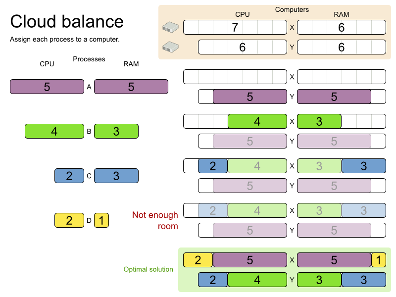
The simple algorithm used here is the First Fit Decreasing algorithm, which assigns the bigger processes first and assigns the smaller processes to the remaining space. As you can see, it is not optimal, because it does not leave enough room to assign the yellow process D.
OptaPlanner finds a more optimal solution by using additional, smarter algorithms. It also scales: both in data (more processes, more computers) and constraints (more hardware requirements, other constraints).
The following summary applies to this example, as well as to an advanced implementation with more constraints that is described in Section 4.7, “Machine reassignment (Google ROADEF 2012)”:
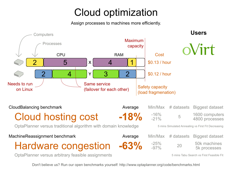
Table 11.1. Cloud balancing problem size
| Problem size | Computers | Processes | Search space |
|---|---|---|---|
| 2computers-6processes | 2 | 6 | 64 |
| 3computers-9processes | 3 | 9 | 10^4 |
| 4computers-012processes | 4 | 12 | 10^7 |
| 100computers-300processes | 100 | 300 | 10^600 |
| 200computers-600processes | 200 | 600 | 10^1380 |
| 400computers-1200processes | 400 | 1200 | 10^3122 |
| 800computers-2400processes | 800 | 2400 | 10^6967 |
11.1.1. Domain Model Design
Using a domain model helps determine which classes are planning entities and which of their properties are planning variables. It also helps to simplify constraints, improve performance, and increase flexibility for future needs.
11.1.1.1. Designing a domain model
To create a domain model, define all the objects that represent the input data for the problem. In this example, the objects are processes and computers.
A separate object in the domain model must represent a full data set of the problem, which contains the input data as well as a solution. In this example, this object holds a list of computers and a list of processes. Each process is assigned to a computer; the distribution of processes between computers is the solution.
Procedure
- Draw a class diagram of your domain model.
- Normalize it to remove duplicate data.
Write down some sample instances for each class. Sample instances are entity properties that are relevant for planning purposes.
Computer: Represents a computer with certain hardware and maintenance costs.In this example, the sample instances for the
Computerclass arecpuPower,memory,networkBandwidth,cost.Process: Represents a process with a demand. Needs to be assigned to aComputerby Planner.Sample instances for
ProcessarerequiredCpuPower,requiredMemory, andrequiredNetworkBandwidth.CloudBalance: Represents the distribution of processes between computers. Contains everyComputerandProcessfor a certain data set.For an object representing the full data set and solution, a sample instance holding the score must be present. OptaPlanner can calculate and compare the scores for different solutions; the solution with the highest score is the optimal solution. Therefore, the sample instance for
CloudBalanceisscore.
Determine which relationships (or fields) change during planning:
Planning entity: The class (or classes) that OptaPlanner can change during solving. In this example, it is the class
Process, because we can move processes to different computers.- A class representing input data that OptaPlanner can not change is known as a problem fact.
-
Planning variable: The property (or properties) of a planning entity class that changes during solving. In this example, it is the property
computeron the classProcess. -
Planning solution: The class that represents a solution to the problem. This class must represent the full data set and contain all planning entities. In this example that is the class
CloudBalance.
In the UML class diagram below, the OptaPlanner concepts are already annotated:
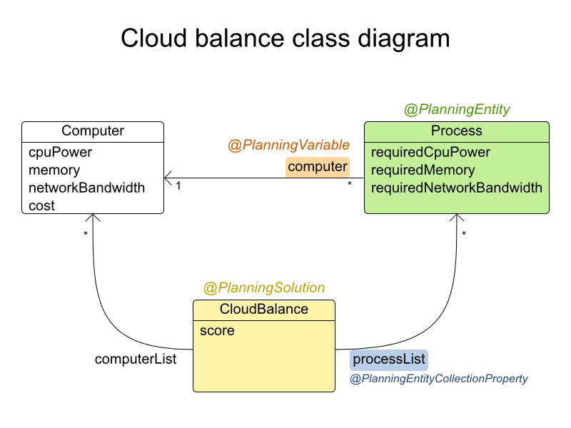
You can find the class definitions for this example in the examples/sources/src/main/java/org/optaplanner/examples/cloudbalancing/domain directory.
11.1.1.2. The Computer Class
The Computer class is a Java object that stores data, sometimes known as a POJO (Plain Old Java Object). Usually, you will have more of this kind of classes with input data.
Example 11.1. CloudComputer.java
public class CloudComputer ... {

    private int cpuPower;
    private int memory;
    private int networkBandwidth;
    private int cost;

    ... // getters
}
11.1.1.3. The Process Class
The Process class is the class that is modified during solving.
We need to tell OptaPlanner that it can change the property computer. To do this, annotate the class with @PlanningEntity and annotate the getComputer() getter with @PlanningVariable.
Of course, the property computer needs a setter too, so OptaPlanner can change it during solving.
Example 11.2. CloudProcess.java
@PlanningEntity(...)
public class CloudProcess ... {

    private int requiredCpuPower;
    private int requiredMemory;
    private int requiredNetworkBandwidth;

    private CloudComputer computer;

    ... // getters

    @PlanningVariable(valueRangeProviderRefs = {"computerRange"})
    public CloudComputer getComputer() {
        return computer;
    }

    public void setComputer(CloudComputer computer) {
        computer = computer;
    }

    // ************************************************************************
    // Complex methods
    // ************************************************************************

    ...

}
OptaPlanner needs to know which values it can choose from to assign to the property computer. Those values are retrieved from the method CloudBalance.getComputerList() on the planning solution, which returns a list of all computers in the current data set.
The @PlanningVariable's valueRangeProviderRefs parameter on CloudProcess.getComputer() needs to match with the @ValueRangeProvider's id on CloudBalance.getComputerList().
You can also use annotations on fields instead of getters.
11.1.1.4. The CloudBalance Class
The CloudBalance class has a @PlanningSolution annotation.
This class holds a list of all computers and processes. It represents both the planning problem and (if it is initialized) the planning solution.
The CloudBalance class has the following key attributes:
It holds a collection of processes that OptaPlanner can change. We annotate the getter
getProcessList()with@PlanningEntityCollectionProperty, so that OptaPlanner can retrieve the processes that it can change. To save a solution, OptaPlanner initializes a new instance of the class with the list of changed processes.-
It also has a
@PlanningScoreannotated propertyscore, which is theScoreof that solution in its current state. OptaPlanner automatically updates it when it calculates aScorefor a solution instance; therefore, this property needs a setter. -
Especially for score calculation with Drools, the property
computerListneeds to be annotated with a@ProblemFactCollectionPropertyso that OptaPlanner can retrieve a list of computers (problem facts) and make it available to the decision engine.
-
It also has a
Example 11.3. CloudBalance.java
@PlanningSolution
public class CloudBalance ... {

    private List<CloudComputer> computerList;

    private List<CloudProcess> processList;

    private HardSoftScore score;

    @ValueRangeProvider(id = "computerRange")
    @ProblemFactCollectionProperty
    public List<CloudComputer> getComputerList() {
        return computerList;
    }

    @PlanningEntityCollectionProperty
    public List<CloudProcess> getProcessList() {
        return processList;
    }

    @PlanningScore
    public HardSoftScore getScore() {
        return score;
    }

    public void setScore(HardSoftScore score) {
        this.score = score;
    }

    ...
}
11.1.2. Running the cloud balancing Hello World application
You can run the sample Hello World application to demonstrate the solver.
Procedure
- Download and configure the examples in your preferred IDE. For instructions on downloading and configuring examples in an IDE, see Section 5.2, “Running the Red Hat build of OptaPlanner examples in an IDE (IntelliJ, Eclipse, or Netbeans)”.
Create a run configuration with the following main class:
org.optaplanner.examples.cloudbalancing.app.CloudBalancingHelloWorldBy default, the Cloud Balancing Hello World is configured to run for 120 seconds.
Result
The application executes the following code:
Example 11.4. CloudBalancingHelloWorld.java
public class CloudBalancingHelloWorld {

    public static void main(String[] args) {
        // Build the Solver
        SolverFactory<CloudBalance> solverFactory = SolverFactory.createFromXmlResource("org/optaplanner/examples/cloudbalancing/solver/cloudBalancingSolverConfig.xml");
        Solver<CloudBalance> solver = solverFactory.buildSolver();

        // Load a problem with 400 computers and 1200 processes
        CloudBalance unsolvedCloudBalance = new CloudBalancingGenerator().createCloudBalance(400, 1200);

        // Solve the problem
        CloudBalance solvedCloudBalance = solver.solve(unsolvedCloudBalance);

        // Display the result
        System.out.println("\nSolved cloudBalance with 400 computers and 1200 processes:\n" + toDisplayString(solvedCloudBalance));
    }

    ...
}
The code example does the following:
Builds the
Solverbased on a solver configuration (in this case an XML file,cloudBalancingSolverConfig.xml, from the classpath).Building the
Solveris the most complicated part of this procedure. For more details, see Section 11.1.3, “Solver Configuration”.SolverFactory<CloudBalance> solverFactory = SolverFactory.createFromXmlResource( "org/optaplanner/examples/cloudbalancing/solver/cloudBalancingSolverConfig.xml"); Solver solver<CloudBalance> = solverFactory.buildSolver();Loads the problem.
CloudBalancingGeneratorgenerates a random problem: you will replace this with a class that loads a real problem, for example from a database.CloudBalance unsolvedCloudBalance = new CloudBalancingGenerator().createCloudBalance(400, 1200);
Solve the problem.
CloudBalance solvedCloudBalance = solver.solve(unsolvedCloudBalance);
Displays the result.
        System.out.println("\nSolved cloudBalance with 400 computers and 1200 processes:\n"
                + toDisplayString(solvedCloudBalance));
11.1.3. Solver Configuration
The solver configuration file determines how the solving process works; it is considered a part of the code. The file is named examples/sources/src/main/resources/org/optaplanner/examples/cloudbalancing/solver/cloudBalancingSolverConfig.xml.
Example 11.5. cloudBalancingSolverConfig.xml
<?xml version="1.0" encoding="UTF-8"?>
<solver>
  <!-- Domain model configuration -->
  <scanAnnotatedClasses/>

  <!-- Score configuration -->
  <scoreDirectorFactory>
    <easyScoreCalculatorClass>org.optaplanner.examples.cloudbalancing.optional.score.CloudBalancingEasyScoreCalculator</easyScoreCalculatorClass>
    <!--<scoreDrl>org/optaplanner/examples/cloudbalancing/solver/cloudBalancingScoreRules.drl</scoreDrl>-->
  </scoreDirectorFactory>

  <!-- Optimization algorithms configuration -->
  <termination>
    <secondsSpentLimit>30</secondsSpentLimit>
  </termination>
</solver>
This solver configuration consists of three parts:
Domain model configuration: What can OptaPlanner change?
We need to make OptaPlanner aware of our domain classes. In this configuration, it will automatically scan all classes in your classpath (for a
@PlanningEntityor@PlanningSolutionannotation):<scanAnnotatedClasses/>
Score configuration: How should OptaPlanner optimize the planning variables? What is our goal?
Since we have hard and soft constraints, we use a
HardSoftScore. But we need to tell OptaPlanner how to calculate the score, depending on our business requirements. Further down, we will look into two alternatives to calculate the score: using a basic Java implementation and using Drools DRL.<scoreDirectorFactory> <easyScoreCalculatorClass>org.optaplanner.examples.cloudbalancing.optional.score.CloudBalancingEasyScoreCalculator</easyScoreCalculatorClass> <!--<scoreDrl>org/optaplanner/examples/cloudbalancing/solver/cloudBalancingScoreRules.drl</scoreDrl>--> </scoreDirectorFactory>Optimization algorithms configuration: How should OptaPlanner optimize it? In this case, we use the default optimization algorithms (because no explicit optimization algorithms are configured) for 30 seconds:
  <termination>
    <secondsSpentLimit>30</secondsSpentLimit>
  </termination>
OptaPlanner should get a good result in seconds (and even in less than 15 milliseconds if the real-time planning feature is used), but the more time it has, the better the result will be. Advanced use cases might use different termination criteria than a hard time limit.
The default algorithms will already easily surpass human planners and most in-house implementations. You can use the advanced Benchmarker feature to power tweak to get even better results.
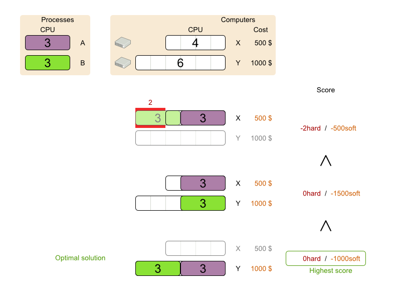
11.1.4. Score Configuration
OptaPlanner will search for the Solution with the highest Score. This example uses a HardSoftScore, which means OptaPlanner will look for the solution with no hard constraints broken (fulfill hardware requirements) and as little as possible soft constraints broken (minimize maintenance cost).
You can define constraints using plain Java, Drools, or the OptaPlanner ConstraintStream API. For information about the ConstraintStream API, see Section 10.3, “Define the constraints and calculate the score”.
11.1.4.1. Configuring score calculation using Java
One way to define a score function is to implement the interface EasyScoreCalculator in plain Java.
Procedure
In the
cloudBalancingSolverConfig.xmlfile, add or uncomment the setting:<scoreDirectorFactory> <easyScoreCalculatorClass>org.optaplanner.examples.cloudbalancing.optional.score.CloudBalancingEasyScoreCalculator</easyScoreCalculatorClass> </scoreDirectorFactory>Implement the
calculateScore(Solution)method to return aHardSoftScoreinstance.Example 11.6. CloudBalancingEasyScoreCalculator.java
public class CloudBalancingEasyScoreCalculator implements EasyScoreCalculator<CloudBalance> {

    /**
     * A very simple implementation. The double loop can easily be removed by using Maps as shown in
     * {@link CloudBalancingMapBasedEasyScoreCalculator#calculateScore(CloudBalance)}.
     */
    public HardSoftScore calculateScore(CloudBalance cloudBalance) {
        int hardScore = 0;
        int softScore = 0;
        for (CloudComputer computer : cloudBalance.getComputerList()) {
            int cpuPowerUsage = 0;
            int memoryUsage = 0;
            int networkBandwidthUsage = 0;
            boolean used = false;

            // Calculate usage
            for (CloudProcess process : cloudBalance.getProcessList()) {
                if (computer.equals(process.getComputer())) {
                    cpuPowerUsage += process.getRequiredCpuPower();
                    memoryUsage += process.getRequiredMemory();
                    networkBandwidthUsage += process.getRequiredNetworkBandwidth();
                    used = true;
                }
            }

            // Hard constraints
            int cpuPowerAvailable = computer.getCpuPower() - cpuPowerUsage;
            if (cpuPowerAvailable < 0) {
                hardScore += cpuPowerAvailable;
            }
            int memoryAvailable = computer.getMemory() - memoryUsage;
            if (memoryAvailable < 0) {
                hardScore += memoryAvailable;
            }
            int networkBandwidthAvailable = computer.getNetworkBandwidth() - networkBandwidthUsage;
            if (networkBandwidthAvailable < 0) {
                hardScore += networkBandwidthAvailable;
            }

            // Soft constraints
            if (used) {
                softScore -= computer.getCost();
            }
        }
        return HardSoftScore.valueOf(hardScore, softScore);
    }

}
Even if we optimize the code above to use Maps to iterate through the processList only once, it is still slow because it does not do incremental score calculation.
To fix that, either use incremental Java score calculation or Drools score calculation. Incremental Java score calculation is not covered in this guide.
11.1.4.2. Configuring score calculation using Drools
You can use Drools rule language (DRL) to define constraints. Drools score calculation uses incremental calculation, where every score constraint is written as one or more score rules.
Using the decision engine for score calculation enables you to integrate with other Drools technologies, such as decision tables (XLS or web based), Business Central, and other supported features.
Procedure
Add a
scoreDrlresource in the classpath to use the decision engine as a score function. In thecloudBalancingSolverConfig.xmlfile, add or uncomment the setting:<scoreDirectorFactory> <scoreDrl>org/optaplanner/examples/cloudbalancing/solver/cloudBalancingScoreRules.drl</scoreDrl> </scoreDirectorFactory>Create the hard constraints. These constraints ensure that all computers have enough CPU, RAM and network bandwidth to support all their processes:
Example 11.7. cloudBalancingScoreRules.drl - Hard Constraints
...

import org.optaplanner.examples.cloudbalancing.domain.CloudBalance;
import org.optaplanner.examples.cloudbalancing.domain.CloudComputer;
import org.optaplanner.examples.cloudbalancing.domain.CloudProcess;

global HardSoftScoreHolder scoreHolder;

// ############################################################################
// Hard constraints
// ############################################################################

rule "requiredCpuPowerTotal"
    when
        $computer : CloudComputer($cpuPower : cpuPower)
        accumulate(
            CloudProcess(
                computer == $computer,
                $requiredCpuPower : requiredCpuPower);
            $requiredCpuPowerTotal : sum($requiredCpuPower);
            $requiredCpuPowerTotal > $cpuPower
        )
    then
        scoreHolder.addHardConstraintMatch(kcontext, $cpuPower - $requiredCpuPowerTotal);
end

rule "requiredMemoryTotal"
    ...
end

rule "requiredNetworkBandwidthTotal"
    ...
end
Create a soft constraint. This constraint minimizes the maintenance cost. It is applied only if hard constraints are met:
Example 11.8. cloudBalancingScoreRules.drl - Soft Constraints
// ############################################################################
// Soft constraints
// ############################################################################

rule "computerCost"
    when
        $computer : CloudComputer($cost : cost)
        exists CloudProcess(computer == $computer)
    then
        scoreHolder.addSoftConstraintMatch(kcontext, - $cost);
end
11.1.5. Further development of the solver
Now that this example works, you can try developing it further. For example, you can enrich the domain model and add extra constraints such as these:
-
Each
Processbelongs to aService. A computer might crash, so processes running the same service should (or must) be assigned to different computers. -
Each
Computeris located in aBuilding. A building might burn down, so processes of the same services should (or must) be assigned to computers in different buildings.