
Data Grid Performance and Sizing Guide
Plan and size Data Grid deployments
Abstract
Red Hat Data Grid
Data Grid is a high-performance, distributed in-memory data store.
- Schemaless data structure
- Flexibility to store different objects as key-value pairs.
- Grid-based data storage
- Designed to distribute and replicate data across clusters.
- Elastic scaling
- Dynamically adjust the number of nodes to meet demand without service disruption.
- Data interoperability
- Store, retrieve, and query data in the grid from different endpoints.
Data Grid documentation
Documentation for Data Grid is available on the Red Hat customer portal.
Data Grid downloads
Access the Data Grid Software Downloads on the Red Hat customer portal.
You must have a Red Hat account to access and download Data Grid software.
Making open source more inclusive
Red Hat is committed to replacing problematic language in our code, documentation, and web properties. We are beginning with these four terms: master, slave, blacklist, and whitelist. Because of the enormity of this endeavor, these changes will be implemented gradually over several upcoming releases. For more details, see our CTO Chris Wright’s message.
Chapter 1. Data Grid deployment models and use cases
Data Grid offers flexible deployment models that support a variety of use cases.
- Drastically improve performance of Red Hat Build of Quarkus, Red Hat JBoss EAP, and Spring applications.
- Ensure service availability and continuity.
- Lower operational costs.
1.1. Data Grid deployment models
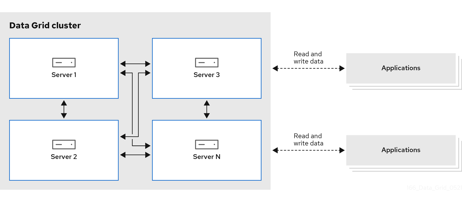
Data Grid has two deployment models for caches, remote and embedded. Both deployment models allow applications to access data with significantly lower latency for read operations and higher throughput for write operations in comparison with traditional database systems.
- Remote caches
- Data Grid Server nodes run in a dedicated Java Virtual Machine (JVM). Clients access remote caches using either Hot Rod, a binary TCP protocol, or REST over HTTP.
- Embedded caches
- Data Grid runs in the same JVM as your Java application, meaning that data is stored in the memory space where code is executed.
Red Hat recommends a server/client architecture for the majority of deployments. Time to deployment is much faster with remote caches because the data layer is separated from business logic. Data Grid Server also provides monitoring and observability and other built-in capabilities to help you lower development costs.
Near-caching
Near-caching capabilities allow remote clients to store data locally, which means read-intensive applications do not need to traverse the network with each call. Near-caching significantly increases speed of read operations and achieves the same performance as an embedded cache.
Figure 1.1. Remote cache deployment model
1.1.1. Platforms and automation tooling
Achieving the desired quality of service means providing Data Grid with optimal CPU and RAM resources. Too few resources downgrades Data Grid performance while using excessive amounts of host resources can quickly increase costs.
While you benchmark and tune Data Grid clusters to find the right allocation of CPU or RAM, you should also consider which host platform provides the right kind of automation tooling to scale clusters and manage resources efficiently.
Bare metal or virtual machine
Couple RHEL, or Microsoft Windows, with Red Hat Ansible to manage Data Grid configuration and poll services to ensure availability and achieve optimal resource usage.
The Ansible collection for Data Grid, available from the Automation Hub, automates cluster installation and includes options for Keycloak integration and cross-site replication.
OpenShift
Take advantage of Kubernetes orchestration to automatically provision pods, impose limits on resources, and automatically scale Data Grid clusters to meet workload demands.
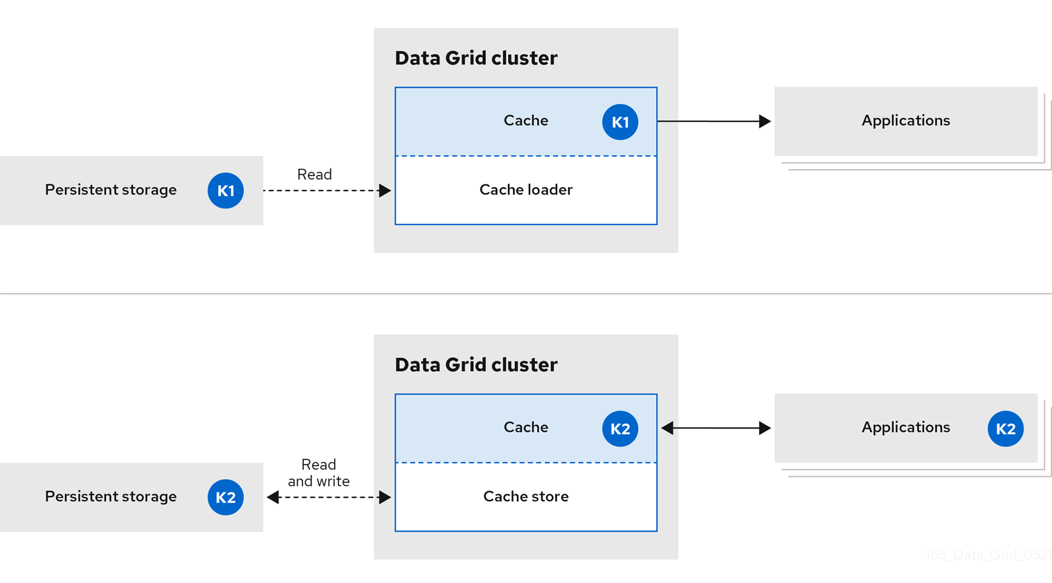
1.2. In-line caching
Data Grid handles all application requests for data that resides in persistent storage.
With in-line caches, Data Grid uses cache loaders and cache stores to operate on data in persistent storage.
- Cache loaders provide read-only access to persistent storage.
- Cache stores provide read and write access to persistent storage.
Figure 1.2. In-line caches
1.3. Side caching
Data Grid stores data that applications retrieve from persistent storage, which reduces the number of read operations to persistent storage and increases response times for subsequent reads.
Figure 1.3. Side caches

With side caches, applications control how data is added to Data Grid clusters from persistent storage. When an application requests an entry, the following occurs:
- The read request goes to Data Grid.
- If the entry is not in the cache, the application requests it from persistent storage.
- The application puts the entry in the cache.
- The application retrieves the entry from Data Grid on the next read.
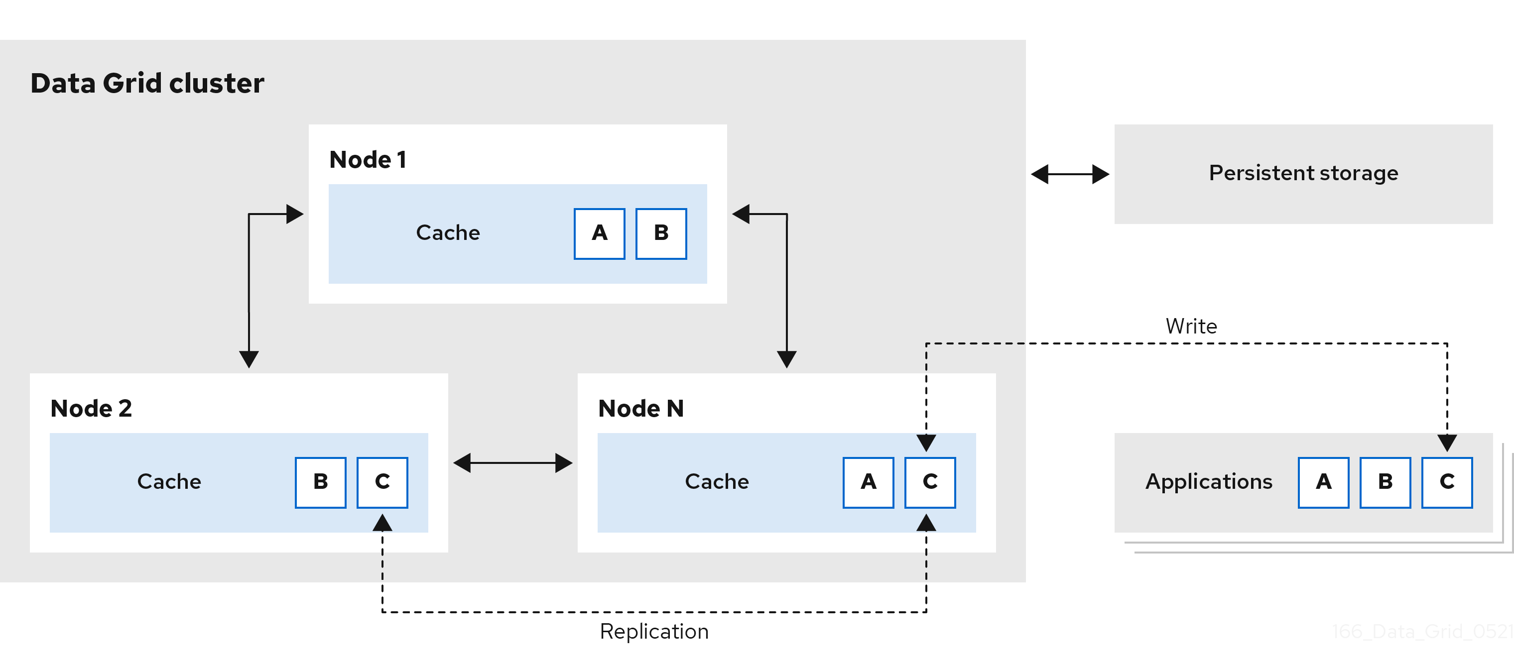
1.4. Distributed memory
Data Grid uses consistent hashing techniques to store a fixed number of copies of each entry in the cache across the cluster. Distributed caches allow you to scale the data layer linearly, increasing capacity as nodes join.
Distributed caches add redundancy to Data Grid clusters to provide fault tolerance and durability guarantees. Data Grid deployments typically configure integration with persistent storage to preserve cluster state for graceful shutdowns and restore from backup.
Figure 1.4. Distributed caches
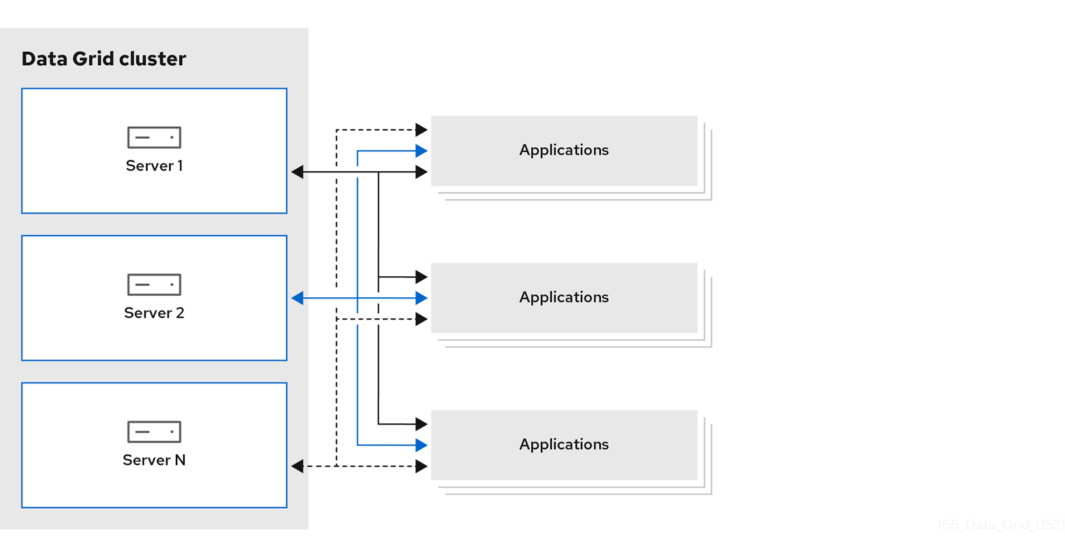
1.5. Session externalization
Data Grid can provide external caches for applications built on Red Hat Build of Quarkus, Red Hat JBoss EAP, Red Hat JBoss Web Server, and Spring. These external caches store HTTP sessions and other data independently of the application layer.
Externalizing sessions to Data Grid gives you the following benefits:
- Elasticity
- Eliminate the need for rebalancing operations when scaling applications.
- Smaller memory footprints
- Storing session data in external caches reduces overall memory requirements for applications.
Figure 1.5. Session externalization
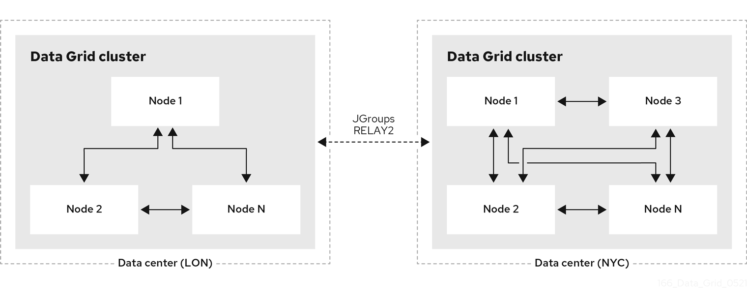
1.6. Cross-site replication
Data Grid can back up data between clusters running in geographically dispersed data centers and across different cloud providers. Cross-site replication provides Data Grid with a global cluster view and:
- Guarantees service continuity in the event of outages or disasters.
- Presents client applications with a single point of access to data in globally distributed caches.
Figure 1.6. Cross-site replication
Chapter 2. Data Grid deployment planning
To get the best performance for your Data Grid deployment, you should do the following things:
- Calculate the size of your data set.
- Determine what type of clustered cache mode best suits your use case and requirements.
- Understand performance trade-offs and considerations for Data Grid capabilities that provide fault tolerance and consistency guarantees.
2.1. Performance metric considerations
Data Grid includes so many configurable combinations that determining a single formula for performance metrics that covers all use cases is not possible.
The purpose of the Data Grid Performance and Sizing Guide document is to provide details about use cases and architectures that can help you determine requirements for your Data Grid deployment.
Additionally, consider the following inter-related factors that apply to Data Grid:
- Available CPU and memory resources in cloud environments
- Caches used in parallel
- Get, put, query balancing
- Peak load and throughput limitations
- Querying limitations with data set
- Number of entries per cache
- Size of cache entries
Given the number of different combinations and unknown external factors, providing a performance calculation that meets all Data Grid use cases is not possible. You cannot compare one performance test to another test if any of the previously listed factors are different.
You can run basic performance tests with the Data Grid CLI that collects limited performance metrics. You can customize the performance test so that the test outputs results that might meet your needs. Test results provide baseline metrics that can help you determine settings and resources for your Data Grid caching requirements.
Measure the performance of your current settings and check if they meet your requirements. If your needs are not met, optimize the settings and then re-measure their performance.
2.2. How to calculate the size of your data set
Planning a Data Grid deployment involves calculating the size of your data set then figuring out the correct number of nodes and amount of RAM to hold the data set.
You can roughly estimate the total size of your data set with this formula:
Data set size = Number of entries * (Average key size + Average value size + Memory overhead)
With remote caches you need to calculate key sizes and value sizes in their marshalled forms.
Data set size in distributed caches
Distributed caches require some additional calculation to determine the data set size.
In normal operating conditions, distributed caches store a number of copies for each key/value entry that is equal to the Number of owners that you configure. During cluster rebalancing operations, some entries have an extra copy, so you should calculate Number of owners + 1 to allow for that scenario.
You can use the following formula to adjust the estimate of your data set size for distributed caches:
Distributed data set size = Data set size * (Number of owners + 1)
Calculating available memory for distributed caches
Distributed caches allow you to increase the data set size either by adding more nodes or by increasing the amount of available memory per node.
Distributed data set size <= Available memory per node * Minimum number of nodes
Adjusting for node loss tolerance
Even if you plan to have a fixed number of nodes in the cluster, you should take into account the fact that not all nodes will be in the cluster all the time. Distributed caches tolerate the loss of Number of owners - 1 nodes without losing data so you can allocate that many extra node in addition to the minimum number of nodes that you need to fit your data set.
Planned nodes = Minimum number of nodes + Number of owners - 1

Distributed data set size <= Available memory per node * (Planned nodes - Number of owners + 1)
For example, you plan to store one million entries that are 10KB each in size and configure three owners per entry for availability. If you plan to allocate 4GB of RAM for each node in the cluster, you can then use the following formula to determine the number of nodes that you need for your data set:
Data set size = 1_000_000 * 10KB = 10GB
Distributed data set size = (3 + 1) * 10GB = 40GB
40GB <= 4GB * Minimum number of nodes
Minimum number of nodes >= 40GB / 4GB = 10
Planned nodes = 10 + 3 - 1 = 12
2.2.1. Memory overhead
Memory overhead is additional memory that Data Grid uses to store entries. An approximate estimate for memory overhead is 200 bytes per entry in JVM heap memory or 60 bytes per entry in off-heap memory. It is impossible to determine a precise amount of memory overhead upfront, however, because the overhead that Data Grid adds per entry depends on several factors. For example, bounding the data container with eviction results in Data Grid using additional memory to keep track of entries. Likewise configuring expiration adds timestamps metadata to each entry.
The only way to find any kind of exact amount of memory overhead involves JVM heap dump analysis. Of course JVM heap dumps provide no information for entries that you store in off-heap memory but memory overhead is much lower for off-heap memory than JVM heap memory.
Additional memory usage
In addition to the memory overhead that Data Grid imposes per entry, processes such as rebalancing and indexing can increase overall memory usage. Rebalancing operations for clusters when nodes join and leave also temporarily require some extra capacity to prevent data loss while replicating entries between cluster members.
2.2.2. JVM heap space allocation
Determine the volume of memory that you require for your Data Grid deployment, so that you have enough data storage capacity to meet your needs.
Allocating a large memory heap size in combination with setting garbage collection (GC) times might impact the performance of your Data Grid deployment in the following ways:
- If a JVM handles only one thread, the GC might block the thread and reduce the JVM’s performance. The GC might operate ahead of the deployment. This asynchronous behavior might cause large GC pauses.
- If CPU resources are low and GC operates synchronously with the deployment, GC might require more frequent runs that can degrade your deployment’s performance.
The following table outlines two examples of allocating JVM heap space for data storage. These examples represent safe estimates for deploying a cluster.
| Cache operations only, such as read, write, and delete operations. | Allocate 50% of JVM heap space for data storage |
| Cache operations and data processing, such as queries and cache event listeners. | Allocate 33% of JVM heap space for data storage |
Depending on pattern changes and usage for data storage, you might consider setting a different percentage for JVM heap space than any of the suggested safe estimates.
Consider setting a safe estimate before you start your Data Grid deployment. After you start your deployment, check the performance of your JVM and the occupancy of heap space. You might need to re-adjust JVM heap space when data usage and throughput for your JVM significantly increases.
The safe estimates were calculated on the assumption that the following common operations were running inside a JVM. The list is not exhaustive, and you might set one of these safe estimates with the purpose of performing additional operations.
- Data Grid converts objects in serialized form to key-value pairs. Data Grid adds the pairs to caches and persistent storage.
- Data Grid encrypts and decrypts caches from remote connections to clients.
- Data Grid performs regular querying of caches to collect data.
- Data Grid strategically divides data into segments to ensure efficient distribution of data among clusters, even during a state transfer operation.
- GC performs more frequent garbage collections, because the JVM allocated large volumes of memory for GC operations.
- GC dynamically manages and monitors data objects in JVM heap space to ensure safe removal of unused objects.
Consider the following factors when allocating JVM heap space for data storage, and when determining the volume of memory and CPU requirements for your Data Grid deployment:
- Clustered cache mode.
Number of segments.
- For example, a low number of segments might affect how a server distributes data among nodes.
- Read or write operations.
Rebalancing requirements.
- For example, a high number of threads might quickly run in parallel during a state transfer, but each thread operation might use more memory.
- Scaling clusters.
- Synchronous or asynchronous replication.
Most notable Data Grid operations that require high CPU resources include rebalancing nodes after pod restarts, running indexing queries on data, and performing GC operations.
Off-heap storage
Data Grid uses JVM heap representations of objects to process read and write operations on caches or perform other operations, such as a state transfer operation. You must always allocate some JVM heap space to Data Grid, even if you store entries in off-heap memory.
The volume of JVM heap memory that Data Grid uses with off-heap storage is much smaller when compared with storing data in the JVM heap space. The JVM heap memory requirements for off-heap storage scales with the number of concurrent operations as against the number of stored entries.
Data Grid uses topology caches to provide clients with a cluster view.
If you receive any OutOfMemoryError exceptions from your Data Grid cluster, consider the options:
- Disable the state transfer operation, which might results in data loss if a node joins or leaves a cluster.
- Recalculate the JVM heap space by factoring in the key size and the number of nodes and segments.
- Use more nodes to better manage memory consumption for your cluster.
- Use a single node, because this might use less memory. However, consider the impact if you want to scale your cluster to its original size.
2.3. Clustered cache modes
You can configure clustered Data Grid caches as replicated or distributed.
- Distributed caches
- Maximize capacity by creating fewer copies of each entry across the cluster.
- Replicated caches
- Provide redundancy by creating a copy of all entries on each node in the cluster.
Reads:Writes
Consider whether your applications perform more write operations or more read operations. In general, distributed caches offer the best performance for writes while replicated caches offer the best performance for reads.
To put k1 in a distributed cache on a cluster of three nodes with two owners, Data Grid writes k1 twice. The same operation in a replicated cache means Data Grid writes k1 three times. The amount of additional network traffic for each write to a replicated cache is equal to the number of nodes in the cluster. A replicated cache on a cluster of ten nodes results in a tenfold increase in traffic for writes and so on. You can minimize traffic by using a UDP stack with multicasting for cluster transport.
To get k1 from a replicated cache, each node can perform the read operation locally. Whereas, to get k1 from a distributed cache, the node that handles the operation might need to retrieve the key from a different node in the cluster, which results in an extra network hop and increases the time for the read operation to complete.
Client intelligence and near-caching
Data Grid uses consistent hashing techniques to make Hot Rod clients topology-aware and avoid extra network hops, which means read operations have the same performance for distributed caches as they do for replicated caches.
Hot Rod clients can also use near-caching capabilities to keep frequently accessed entries in local memory and avoid repeated reads.
Distributed caches are the best choice for most Data Grid Server deployments. You get the best possible performance for read and write operations along with elasticity for cluster scaling.
Data guarantees
Because each node contains all entries, replicated caches provide more protection against data loss than distributed caches. On a cluster of three nodes, two nodes can crash and you do not lose data from a replicated cache.
In that same scenario, a distributed cache with two owners would lose data. To avoid data loss with distributed caches, you can increase the number of replicas across the cluster by configuring more owners for each entry with either the owners attribute declaratively or the numOwners() method programmatically.
Rebalancing operations when node failure occurs
Rebalancing operations after node failure can impact performance and capacity. When a node leaves the cluster, Data Grid replicates cache entries among the remaining members to restore the configured number of owners. This rebalancing operation is temporary, but the increased cluster traffic has a negative impact on performance. Performance degradation is greater the more nodes leave. The nodes left in the cluster might not have enough capacity to keep all data in memory when too many nodes leave.
Cluster scaling
Data Grid clusters scale horizontally as your workloads demand to more efficiently use compute resources like CPU and memory. To take the most advantage of this elasticity, you should consider how scaling the number of nodes up or down affects cache capacity.
For replicated caches, each time a node joins the cluster, it receives a complete copy of the data set. Replicating all entries to each node increases the time it takes for nodes to join and imposes a limit on overall capacity. Replicated caches can never exceed the amount of memory available to the host. For example, if the size of your data set is 10 GB, each node must have at least 10 GB of available memory.
For distributed caches, adding more nodes increases capacity because each member of the cluster stores only a subset of the data. To store 10 GB of data, you can have eight nodes each with 5 GB of available memory if the number of owners is two, without taking memory overhead into consideration. Each additional node that joins the cluster increases the capacity of the distributed cache by 5 GB.
The capacity of a distributed cache is not bound by the amount of memory available to underlying hosts.
Synchronous or asynchronous replication
Data Grid can communicate synchronously or asynchronously when primary owners send replication requests to backup nodes.
| Replication mode | Effect on performance |
|---|---|
| Synchronous | Synchronous replication helps to keep your data consistent but adds latency to cluster traffic that reduces throughput for cache writes. |
| Asynchronous | Asynchronous replication reduces latency and increases the speed of write operations but leads to data inconsistency and provides a lower guarantee against data loss. |
With synchronous replication, Data Grid notifies the originating node when replication requests complete on backup nodes. Data Grid retries the operation if a replication request fails due to a change to the cluster topology. When replication requests fail due to other errors, Data Grid throws exceptions for client applications.
With asynchronous replication, Data Grid does not provide any confirmation for replication requests. This has the same effect for applications as all requests being successful. On the Data Grid cluster, however, the primary owner has the correct entry and Data Grid replicates it to backup nodes at some point in the future. In the case that the primary owner crashes then backup nodes might not have a copy of the entry or they might have an out of date copy.
Cluster topology changes can also lead to data inconsistency with asynchronous replication. For example, consider a Data Grid cluster that has multiple primary owners. Due to a network error or some other issue, one or more of the primary owners leaves the cluster unexpectedly so Data Grid updates which nodes are the primary owners for which segments. When this occurs, it is theoretically possible for some nodes to use the old cluster topology and some nodes to use the updated topology. With asynchronous communication, this might lead to a short time where Data Grid processes replication requests from the previous topology and applies older values from write operations. However, Data Grid can detect node crashes and update cluster topology changes quickly enough that this scenario is not likely to affect many write operations.
Using asynchronous replication does not guarantee improved throughput for writes, because asynchronous replication limits the number of backup writes that a node can handle at any time to the number of possible senders (via JGroups per-sender ordering). Synchronous replication allows nodes to handle more incoming write operations at the same time, which in certain configurations might compensate for the fact that individual operations take longer to complete, giving you a higher total throughput.
When a node sends multiple requests to replicate entries, JGroups sends the messages to the rest of the nodes in the cluster one at a time, which results in there being only one replication request per originating node. This means that Data Grid nodes can process, in parallel with other write operations, one write from each other node in the cluster.
Data Grid uses a JGroups flow control protocol in the cluster transport layer to handle replication requests to backup nodes. If the number of unconfirmed replication requests exceeds the flow control threshold, set with the max_credits attribute (4MB by default), write operations are blocked on the originator node. This applies to both synchronous and asynchronous replication.
Number of segments
Data Grid divides data into segments to distribute data evenly across clusters. Even distribution of segments avoids overloading individual nodes and makes cluster re-balancing operations more efficient.
Data Grid creates 256 hash space segments per cluster by default. For deployments with up to 20 nodes per cluster, this number of segments is ideal and should not change.
For deployments with greater than 20 nodes per cluster, increasing the number of segments increases the granularity of your data so Data Grid can distribute it across the cluster more efficiently. Use the following formula to calculate approximately how many segments you should configure:
Number of segments = 20 * Number of nodes
For example, with a cluster of 30 nodes you should configure 600 segments. Adding more segments for larger clusters is generally a good idea, though, and this formula should provide you with a rough idea of the number that is right for your deployment.
Changing the number of segments Data Grid creates requires a full cluster restart. If you use persistent storage you might also need to use the StoreMigrator utility to change the number of segments, depending on the cache store implementation.
Changing the number of segments can also lead to data corruption so you should do so with caution and based on metrics that you gather from benchmarking and performance monitoring.
Data Grid always segments data that it stores in memory. When you configure cache stores, Data Grid does not always segment data in persistent storage.
It depends on the cache store implementation but, whenever possible you should enable segmentation for a cache store. Segmented cache stores improve Data Grid performance when iterating over data in persistent storage. For example, with RocksDB and JDBC-string based cache stores, segmentation reduces the number of objects that Data Grid needs to retrieve from the database.
2.4. Strategies to manage stale data
If Data Grid is not the primary source of data, embedded and remote caches are stale by nature. While planning, benchmarking, and tuning your Data Grid deployment, choose the appropriate level of cache staleness for your applications.
Choose a level that allows you to make the best use of available RAM and avoid cache misses. If Data Grid does not have the entry in memory, then calls go to the primary store when applications send read and write requests.
Cache misses increase the latency of reads and writes but, in many cases, calls to the primary store are more costly than the performance penalty to Data Grid. One example of this is offloading relational database management systems (RDBMS) to Data Grid clusters. Deploying Data Grid in this way greatly reduces the financial cost of operating traditional databases so tolerating a higher degree of stale entries in caches makes sense.
With Data Grid you can configure maximum idle and lifespan values for entries to maintain an acceptable level of cache staleness.
- Expiration
- Controls how long Data Grid keeps entries in a cache and takes effect across clusters.
Higher expiration values mean that entries remain in memory for longer, which increases the likelihood that read operations return stale values. Lower expiration values mean that there are less stale values in the cache but the likelihood of cache misses is greater.
To carry out expiration, Data Grid creates a reaper from the existing thread pool. The main performance consideration with the thread is configuring the right interval between expiration runs. Shorter intervals perform more frequent expiration but use more threads.
Additionally, with maximum idle expiration, you can control how Data Grid updates timestamp metadata across clusters. Data Grid sends touch commands to coordinate maximum idle expiration across nodes synchronously or asynchronously. With synchronous replication, you can choose either "sync" or "async" touch commands depending on whether you prefer consistency or speed.
2.5. JVM memory management with eviction
RAM is a costly resource and usually limited in availability. Data Grid lets you manage memory usage to give priority to frequently used data by removing entries from memory.
- Eviction
- Controls the amount of data that Data Grid keeps in memory and takes effect for each node.
Eviction bounds Data Grid caches by:
- Total number of entries, a maximum count.
- Amount of JVM memory, a maximum size.
Data Grid evicts entries on a per-node basis. Because not all nodes evict the same entries you should use eviction with persistent storage to avoid data inconsistency.
The impact to performance from eviction comes from the additional processing that Data Grid needs to calculate when the size of a cache reaches the configured threshold.
Eviction can also slow down read operations. For example, if a read operation retrieves an entry from a cache store, Data Grid brings that entry into memory and then evicts another entry. This eviction process can include writing the newly evicted entry to the cache store, if using passivation. When this happens, the read operation does not return the value until the eviction process is complete.
2.6. JVM heap and off-heap memory
Data Grid stores cache entries in JVM heap memory by default. You can configure Data Grid to use off-heap storage, which means that your data occupies native memory outside the managed JVM memory space.
The following diagram is a simplified illustration of the memory space for a JVM process where Data Grid is running:
Figure 2.1. JVM memory space
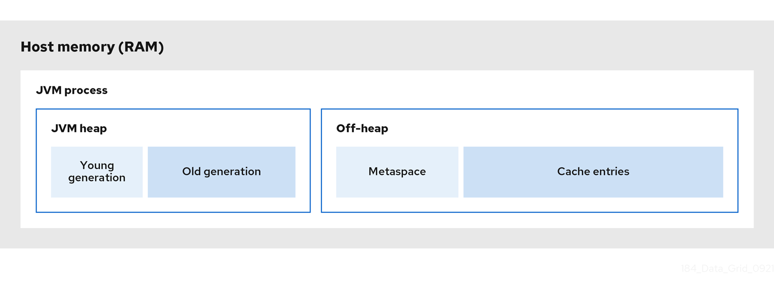
JVM heap memory
The heap is divided into young and old generations that help keep referenced Java objects and other application data in memory. The GC process reclaims space from unreachable objects, running more frequently on the young generation memory pool.
When Data Grid stores cache entries in JVM heap memory, GC runs can take longer to complete as you start adding data to your caches. Because GC is an intensive process, longer and more frequent runs can degrade application performance.
Off-heap memory
Off-heap memory is native available system memory outside JVM memory management. The JVM memory space diagram shows the Metaspace memory pool that holds class metadata and is allocated from native memory. The diagram also represents a section of native memory that holds Data Grid cache entries.
Off-heap memory:
- Uses less memory per entry.
- Improves overall JVM performance by avoiding Garbage Collector (GC) runs.
One disadvantage, however, is that JVM heap dumps do not show entries stored in off-heap memory.
2.6.1. Off-heap data storage
When you add entries to off-heap caches, Data Grid dynamically allocates native memory to your data.
Data Grid hashes the serialized byte[] for each key into buckets that are similar to a standard Java HashMap. Buckets include address pointers that Data Grid uses to locate entries that you store in off-heap memory.
Even though Data Grid stores cache entries in native memory, run-time operations require JVM heap representations of those objects. For instance, cache.get() operations read objects into heap memory before returning. Likewise, state transfer operations hold subsets of objects in heap memory while they take place.
Object equality
Data Grid determines equality of Java objects in off-heap storage using the serialized byte[] representation of each object instead of the object instance.
Data consistency
Data Grid uses an array of locks to protect off-heap address spaces. The number of locks is twice the number of cores and then rounded to the nearest power of two. This ensures that there is an even distribution of ReadWriteLock instances to prevent write operations from blocking read operations.
2.7. Persistent storage
Configuring Data Grid to interact with a persistent data source greatly impacts performance. This performance penalty comes from the fact that more traditional data sources are inherently slower than in-memory caches. Read and write operations will always take longer when the call goes outside the JVM. Depending on how you use cache stores, though, the reduction of Data Grid performance is offset by the performance boost that in-memory data provides over accessing data in persistent storage.
Configuring Data Grid deployments with persistent storage also gives other benefits, such as allowing you to preserve state for graceful cluster shutdowns. You can also overflow data from your caches to persistent storage and gain capacity beyond what is available in memory only. For example, you can have ten million entries in total while keeping only two million of them in memory.
Data Grid adds key/value pairs to caches and persistent storage in either write-through mode or write-behind mode. Because these writing modes have different impacts on performance, you must consider them when planning a Data Grid deployment.
| Writing mode | Effect on performance |
|---|---|
| Write-through | Data Grid writes data to the cache and persistent storage simultaneously, which increases consistency and avoids data loss that can result from node failure.
The downside to write-through mode is that synchronous writes add latency and decrease throughput. |
| Write-behind | Data Grid synchronously writes data to the cache but then adds the modification to a queue so that the write to persistent storage happens asynchronously, which decreases consistency but reduces latency of write operations. When the cache store cannot handle the number of write operations, Data Grid delays new writes until the number of pending write operations goes below the configured modification queue size, in a similar way to write-through. If the store is normally fast enough but latency spikes occur during bursts of cache writes, you can increase the modification queue size to contain the bursts and reduce the latency. |
Passivation
Enabling passivation configures Data Grid to write entries to persistent storage only when it evicts them from memory. Passivation also implies activation. Performing a read or write on a key brings that key back into memory and removes it from persistent storage. Removing keys from persistent storage during activation does not block the read or write operation, but it does increase load on the external store.
Passivation and activation can potentially result in Data Grid performing multiple calls to persistent storage for a given entry in the cache. For example, if an entry is not available in memory, Data Grid brings it back into memory which is one read operation and a delete operation to remove it from persistent storage. Additionally, if the cache has reached the size limit, then Data Grid performs another write operation to passivate a newly evicted entry.
Pre-loading caches with data
Another aspect of persistent storage that can affect Data Grid cluster performance is pre-loading caches. This capability populates your caches with data when Data Grid clusters start so they are "warm" and can handle reads and writes straight away. Pre-loading caches can slow down Data Grid cluster start times and result in out of memory exceptions if the amount of data in persistent storage is greater than the amount of available RAM.
2.8. Cluster security
Protecting your data and preventing network intrusion is one of the most important aspect of deployment planning. Sensitive customer details leaking to the open internet or data breaches that allow hackers to publicly expose confidential information have devastating impacts on business reputation.
With this in mind you need a robust security strategy to authenticate users and encrypt network communication. But what are the costs to the performance of your Data Grid deployment? How should you approach these considerations during planning?
Authentication
The performance cost of validating user credentials depends on the mechanism and protocol. Data Grid validates credentials once per user over Hot Rod while potentially for every request over HTTP.
Table 2.1. Authentication mechanisms
| SASL mechanism | HTTP mechanism | Performance impact |
|---|---|---|
|
|
|
While |
|
|
|
For both Hot Rod and HTTP requests, the
For Hot Rod endpoints, the |
|
|
| A Kerberos server, Key Distribution Center (KDC), handles authentication and issues tokens to users. Data Grid performance benefits from the fact that a separate system handles user authentication operations. However these mechanisms can lead to network bottlenecks depending on the performance of the KDC service itself. |
|
|
| Federated identity providers that implement the OAuth standard for issuing temporary access tokens to Data Grid users. Users authenticate with an identity service instead of directly authenticating to Data Grid, passing the access token as a request header instead. Compared to handling authentication directly, there is a lower performance penalty for Data Grid to validate user access tokens. Similarly to a KDC, actual performance implications depend on the quality of service for the identity provider itself. |
|
|
| You can provide trust stores to Data Grid Server so that it authenticates inbound connections by comparing certificates that clients present against the trust stores. If the trust store contains only the signing certificate, which is typically a Certificate Authority (CA), any client that presents a certificate signed by the CA can connect to Data Grid. This offers lower security and is vulnerable to MITM attacks but is faster than authenticating the public certificate of each client. If the trust store contains all client certificates in addition to the signing certificate, only those clients that present a signed certificate that is present in the trust store can connect to Data Grid. In this case Data Grid compares the common Common Name (CN) from the certificate that the client presents with the trust store in addition to verifying that the certificate is signed, adding more overhead. |
Encryption
Encrypting cluster transport secures data as it passes between nodes and protects your Data Grid deployment from MITM attacks. Nodes perform TLS/SSL handshakes when joining the cluster which carries a slight performance penalty and increased latency with additional round trips. However, once each node establishes a connection it stays up forever assuming connections never go idle.
For remote caches, Data Grid Server can also encrypt network communication with clients. In terms of performance the effect of TLS/SSL connections between clients and remote caches is the same. Negotiating secure connections takes longer and requires some additional work but, once the connections are established latency from encryption is not a concern for Data Grid performance.
Apart from using TLSv1.3, the only means of offsetting performance loss from encryption are to configure the JVM on which Data Grid runs. For instance using OpenSSL libraries instead of standard Java encryption provides more efficient handling with results up to 20% faster.
Authorization
Role-based access control (RBAC) lets you restrict operations on data, offering additional security to your deployments. RBAC is the best way to implement a policy of least privilege for user access to data distributed across Data Grid clusters. Data Grid users must have a sufficient level of authorization to read, create, modify, or remove data from caches.
Adding another layer of security to protect your data will always carry a performance cost. Authorization adds some latency to operations because Data Grid validates each one against an Access Control List (ACL) before allowing users to manipulate data. However the overall impact to performance from authorization is much lower than encryption so the cost to benefit generally balances out.
2.9. Client listeners
Client listeners provide notifications whenever data is added, removed, or modified on your Data Grid cluster.
As an example, the following implementation triggers an event whenever temperatures change at a given location:
@ClientListener
public class TemperatureChangesListener {
   private String location;

   TemperatureChangesListener(String location) {
      this.location = location;
   }

   @ClientCacheEntryCreated
   public void created(ClientCacheEntryCreatedEvent event) {
      if(event.getKey().equals(location)) {
         cache.getAsync(location)
               .whenComplete((temperature, ex) ->
                     System.out.printf(">> Location %s Temperature %s", location, temperature));
      }
   }
}
Adding listeners to Data Grid clusters adds performance considerations for your deployment.
For embedded caches, listeners use the same CPU cores as Data Grid. Listeners that receive many events and use a lot of CPU to process those events reduce the CPU available to Data Grid and slow down all other operations.
For remote caches, Data Grid Server uses an internal process to trigger client notifications. Data Grid Server sends the event from the primary owner node to the node where the listener is registered before sending it to the client. Data Grid Server also includes a backpressure mechanism that delays write operations to caches if client listeners process events too slowly.
Filtering listener events
If listeners are invoked on every write operation, Data Grid can generate a high number of events, creating network traffic both inside the cluster and to external clients. It all depends on how many clients are registered with each listener, the type of events they trigger, and how data changes on your Data Grid cluster.
As an example with remote caches, if you have ten clients registered with a listener that emits 10 events, Data Grid Server sends 100 events in total across the network.
You can provide Data Grid Server with custom filters to reduce traffic to clients. Filters allow Data Grid Server to first process events and determine whether to forward them to clients.
Continuous queries and listeners
Continuous queries allow you to receive events for matching entries and offers an alternative to deploying client listeners and filtering listener events. Of course queries have additional processing costs that you need to take into account but, if you already index caches and perform queries, using a continuous query instead of a client listener could be worthwhile.
2.10. Indexing and querying caches
Querying Data Grid caches lets you analyze and filter data to gain real-time insights. As an example, consider an online game where players compete against each other in some way to score points. If you wanted to implement a leaderboard with the top ten players at any one time, you could create a query to find out which players have the most points at any one time and limit the result to a maximum of ten as follows:
QueryFactory queryFactory = Search.getQueryFactory(playersScores);
Query topTenQuery = queryFactory
  .create("from com.redhat.PlayerScore ORDER BY p.score DESC, p.timestamp ASC")
  .maxResults(10);
List<PlayerScore> topTen = topTenQuery.execute().list();
The preceding example illustrates the benefit of using queries because it lets you find ten entries that match a criteria out of potentially millions of cache entries.
In terms of performance impact, though, you should consider the tradeoffs that come with indexing operations versus query operations. Configuring Data Grid to index caches results in much faster queries. Without indexes, queries must scroll through all data in the cache, slowing down results by orders of magnitude depending on the type and amount of data.
There is a measurable loss of performance for writes when indexing is enabled. However, with some careful planning and a good understanding of what you want to index, you can avoid the worst effects.
The most effective approach is to configure Data Grid to index only the fields that you need. Whether you store Plain Old Java Objects (POJOs) or use Protobuf schema, the more fields that you annotate, the longer it takes Data Grid to build the index. If you have a POJO with five fields but you only need to query two of those fields, do not configure Data Grid to index the three fields you don’t need.
Data Grid gives you several options to tune indexing operations. For instance Data Grid stores indexes differently to data, saving indexes to disk instead of memory. Data Grid keeps the index synchronized with the cache using an index writer, whenever an entry is added, modified or deleted. If you enable indexing and then observe slower writes, and think indexing causes the loss of performance, you can keep indexes in a memory buffer for longer periods of time before writing to disk. This results in faster indexing operations, and helps mitigate degradation of write throughput, but consumes more memory. For most deployments, though, the default indexing configuration is suitable and does not slow down writes too much.
In some scenarios it might be sensible not to index your caches, such as for write-heavy caches that you need to query infrequently and don’t need results in milliseconds. It all depends on what you want to achieve. Faster queries means faster reads but comes at the expense of slower writes that come with indexing.
You can improve performance of indexed queries by setting properly the maxResults and the hit-count-accuracy values.
Additional resources
2.10.1. Continuous queries and Data Grid performance
Continuous queries provide a constant stream of updates to applications, which can generate a significant number of events. Data Grid temporarily allocates memory for each event it generates, which can result in memory pressure and potentially lead to OutOfMemoryError exceptions, especially for remote caches. For this reason, you should carefully design your continuous queries to avoid any performance impact.
Data Grid strongly recommends that you limit the scope of your continuous queries to the smallest amount of information that you need. To achieve this, you can use projections and predicates. For example, the following statement provides results about only a subset of fields that match the criteria rather than the entire entry:
SELECT field1, field2 FROM Entity WHERE x AND y
It is also important to ensure that each ContinuousQueryListener you create can quickly process all received events without blocking threads. To achieve this, you should avoid any cache operations that generate events unnecessarily.
2.11. Data consistency
Data that resides on a distributed system is vulnerable to errors that can arise from temporary network outages, system failures, or just simple human error. These external factors are uncontrollable but can have serious consequences for quality of your data. The effects of data corruption range from lower customer satisfaction to costly system reconciliation that results in service unavailability.
Data Grid can carry out ACID (atomic, consistent, isolated, durable) transactions to ensure the cache state is consistent.
Transactions are a sequence of operations that Data Grid caries out as a single operation. Either all write operations in a transaction complete successfully or they all fail. In this way, the transaction either modifies the cache state in a consistent way, providing a history of reads and writes, or it does not modify cache state at all.
The main performance concern for enabling transactions is finding the balance between having a more consistent data set and increasing latency that degrades write throughput.
Write locks with transactions
Configuring the wrong locking mode can negatively affect the performance of your transactions. The right locking mode depends on whether your Data Grid deployment has a high or low rate of contention for keys.
For workloads with low rates of contention, where two or more transactions are not likely to write to the same key simultaneously, optimistic locking offers the best performance.
Data Grid acquires write locks on keys before transactions commit. If there is contention for keys, the time it takes to acquire locks can delay commits. Additionally, if Data Grid detects conflicting writes, then it rolls the transaction back and the application must retry it, increasing latency.
For workloads with high rates of contention, pessimistic locking provides the best performance.
Data Grid acquires write locks on keys when applications access them to ensure no other transaction can modify the keys. Transaction commits complete in a single phase because keys are already locked. Pessimistic locking with multiple key transactions results in Data Grid locking keys for longer periods of time, which can decrease write throughput.
Read isolation
Isolation levels do not impact Data Grid performance considerations except for optimistic locking with REPEATABLE_READ. With this combination, Data Grid checks for write skews to detect conflicts, which can result in longer transaction commit phases. Data Grid also uses version metadata to detect conflicting write operations, which can increase the amount of memory per entry and generate additional network traffic for the cluster.
Transaction recovery and partition handling
If networks become unstable due to partitions or other issues, Data Grid can mark transactions as "in-doubt". When this happens Data Grid retains write locks that it acquires until the network stabilizes and the cluster returns to a healthy operational state. In some cases it might be necessary for a system administrator to manually complete any "in-doubt" transactions.
2.12. Network partitions and degraded clusters
Data Grid clusters can encounter split brain scenarios where subsets of nodes in the cluster become isolated from each other and communication between nodes becomes disjointed. When this happens, Data Grid caches in minority partitions enter DEGRADED mode while caches in majority partitions remain available.
Garbage collection (GC) pauses are the most common cause of network partitions. When GC pauses result in nodes becoming unresponsive, Data Grid clusters can start operating in a split brain network.
Rather than dealing with network partitions, try to avoid GC pauses by controlling JVM heap usage and by using a modern, low-pause GC implementation such as Shenandoah with OpenJDK.
CAP theorem and partition handling strategies
CAP theorem expresses a limitation of distributed, key/value data stores, such as Data Grid. When network partition events happen, you must choose between consistency or availability while Data Grid heals the partition and resolves any conflicting entries.
- Availability
- Allow read and write operations.
- Consistency
- Deny read and write operations.
Data Grid can also allow reads only while joining clusters back together. This strategy is a more balanced option of consistency by denying writes to entries and availability by allowing applications to access (potentially stale) data.
Removing partitions
As part of the process of joining the cluster back together and returning to normal operations, Data Grid resolves conflicting entries according to a merge policy.
By default Data Grid does not attempt to resolve conflicts on merge which means clusters return to a healthy state sooner and there is no performance penalty beyond normal cluster rebalancing. However, in this case, data in the cache is much more likely to be inconsistent.
If you configure a merge policy then it takes much longer for Data Grid to heal partitions. Configuring a merge policy results in Data Grid retrieving every version of an entry from each cache and then resolving any conflicts as follows:
|
| Data Grid finds the value that exists on the majority of nodes in the cluster and applies it, which can restore out of date values. |
|
| Data Grid applies the first non-null value that it finds on the cluster, which can restore out of date values. |
|
| Data Grid removes any entries that have conflicting values. |
2.12.1. Garbage collection and partition handling
Long garbage collection (GC) times can increase the amount of time it takes Data Grid to detect network partitions. In some cases, GC can cause Data Grid to exceed the maximum time to detect a split.
Additionally, when merging partitions after a split, Data Grid attempts to confirm all nodes are present in the cluster. Because no timeout or upper bound applies to the response time from nodes, the operation to merge the cluster view can be delayed. This can result from network issues as well as long GC times.
Another scenario in which GC can impact performance through partition handling is when GC suspends the JVM, causing one or more nodes to leave the cluster. When this occurs, and suspended nodes resume after GC completes, the nodes can have out of date or conflicting cluster topologies.
If a merge policy is configured, Data Grid attempts to resolve conflicts before merging the nodes. However, the merge policy is used only if the nodes have incompatible consistent hashes. Two consistent hashes are compatible if they have at least one common owner for each segment or incompatible if they have no common owner for at least one segment.
When nodes have old, but compatible, consistent hashes, Data Grid ignores the out of date cluster topology and does not attempt to resolve conflicts. For example, if one node in the cluster is suspended due to garbage collection (GC), other nodes in the cluster remove it from the consistent hash and replace it with new owner nodes. If numOwners > 1, the old consistent hash and the new consistent hash have a common owner for every key, which makes them compatible and allows Data Grid to skip the conflict resolution process.
2.13. Cluster backups and disaster recovery
Data Grid clusters that perform cross-site replication are typically "symmetrical" in terms of overall CPU and memory allocation. When you take cross-site replication into account for sizing, the primary concern is the impact of state transfer operations between clusters.
For example, a Data Grid cluster in NYC goes offline and clients switch to a Data Grid cluster in LON. When the cluster in NYC comes back online, state transfer occurs from LON to NYC. This operation prevents stale reads from clients but has a performance penalty for the cluster that receives state transfer.
You can distribute the increase in processing that state transfer operations require across the cluster. However the performance impact from state transfer operations depends entirely on the environment and factors such as the type and size of the data set.
Conflict resolution for Active/Active deployments
Data Grid detects conflicts with concurrent write operations when multiple sites handle client requests, known as an Active/Active site configuration.
The following example illustrates how concurrent writes result in a conflicting entry for Data Grid clusters running in the LON and NYC data centers:
            LON       NYC

k1=(n/a)    0,0       0,0

k1=2        1,0  -->  1,0   k1=2

k1=3        1,1  <--  1,1   k1=3

k1=5        2,1       1,2   k1=8

                 -->  2,1 (conflict)
(conflict)  1,2  <--
In an Active/Active site configuration, you should never use the synchronous backup strategy because concurrent writes result in deadlocks and you lose data. With the asynchronous backup strategy (strategy=async), Data Grid gives you a choice cross-site merge policies for handling concurrent writes.
In terms of performance, merge policies that Data Grid uses to resolve conflicts do require additional computation but generally do not incur a significant penalty. For instance the default cross-site merge policy uses a lexicographic comparison, or "string comparison", that only takes a couple of nanoseconds to complete.
Data Grid also provides a XSiteEntryMergePolicy SPI for cross-site merge policies. If you do configure Data Grid to resolve conflicts with a custom implementation you should always monitor performance to gauge any adverse effects.
The XSiteEntryMergePolicy SPI invokes all merge policies in the non-blocking thread pool. If you implement a blocking custom merge policy, it can exhaust the thread pool.
You should delegate complex or blocking policies to a different thread and your implementation should return a CompletionStage that completes when the merge policy is done in the other thread.
2.14. Code execution and data processing
One of the benefits of distributed caching is that you can leverage compute resources from each host to perform large scale data processing more efficiently. By executing your processing logic directly on Data Grid you spread the workload across multiple JVM instances. Your code also runs in the same memory space where Data Grid stores your data, meaning that you can iterate over entries much faster.
In terms of performance impact to your Data Grid deployment, that entirely depends on your code execution. More complex processing operations have higher performance penalties so you should approach running any code on Data Grid clusters with careful planning. Start out by testing your code and performing multiple execution runs on a smaller, sample data set. After you gather some metrics you can start identifying optimizations and understanding what performance implications of the code you’re running.
One definite consideration is that long running processes can start having a negative impact on normal read and write operations. So it is imperative that you monitor your deployment over time and continually assess performance.
Embedded caches
With embedded caches, Data Grid provides two APIs that let you execute code in the same memory space as your data.
ClusterExecutorAPI- Lets you perform any operation with the Cache Manager, including iterating over the entries of one or more caches, and gives you processing based on Data Grid nodes.
CacheStreamAPI- Lets you perform operations on collections and gives you processing based on data.
If you want to run an operation on a single node, a group of nodes, or all nodes in a certain geographic region, then you should use clustered execution. If you want to run an operation that guarantees a correct result for your entire data set, then using distributed streams is a more effective option.
Cluster execution
ClusterExecutor clusterExecutor = cacheManager.executor();
clusterExecutor.singleNodeSubmission().filterTargets(policy);
for (int i = 0; i < invocations; ++i) {
   clusterExecutor.submitConsumer((cacheManager) -> {
      TransportConfiguration tc =
      cacheManager.getCacheManagerConfiguration().transport();
      return tc.siteId() + tc.rackId() + tc.machineId();
   }, triConsumer).get(10, TimeUnit.SECONDS);
}
CacheStream
Map<Object, String> jbossValues =
cache.entrySet().stream()
     .filter(e -> e.getValue().contains("JBoss"))
     .collect(Collectors.toMap(Map.Entry::getKey, Map.Entry::getValue));
Additional resources
Remote caches
For remote caches, Data Grid provides a ServerTask API that lets you register custom Java implementations with Data Grid Server and execute tasks programmatically by calling the execute() method over Hot Rod or by using the Data Grid Command Line Interface (CLI). You can execute tasks on one Data Grid Server instance only or all server instances in the cluster.
2.15. Client traffic
When sizing remote Data Grid clusters, you need to calculate the number and size of entries but also the amount of client traffic. Data Grid needs enough RAM to store your data and enough CPU to handle client read and write requests in a timely manner.
There are many different factors that affect latency and determine response times. For example, the size of the key/value pair affects the response time for remote caches. Other factors that affect remote cache performance include the number of requests per second that the cluster receives, the number of clients, as well as the ratio of read operations to write operations.
Chapter 3. Benchmarking Data Grid on OpenShift
For Data Grid clusters running on OpenShift, Red Hat recommends using Hyperfoil to measure performance. Hyperfoil is a benchmarking framework that provides accurate performance results for distributed services.
3.1. Benchmarking Data Grid
After you set up and configure your deployment, start benchmarking your Data Grid cluster to analyze and measure performance. Benchmarking shows you where limits exist so you can adjust your environment and tune your Data Grid configuration to get the best performance, which means achieving the lowest latency and highest throughput possible.
It is worth noting that optimal performance is a continual process, not an ultimate goal. When your benchmark tests show that your Data Grid deployment has reached a desired level of performance, you cannot expect those results to be fixed or always valid.
3.2. Installing Hyperfoil
Set up Hyperfoil on Red Hat OpenShift by creating an operator subscription and downloading the Hyperfoil distribution that includes the command line interface (CLI).
Procedure
Create a Hyperfoil Operator subscription through the OperatorHub in the OpenShift Web Console.
NoteHyperfoil Operator is available as a Community Operator.
Red Hat does not certify the Hyperfoil Operator and does not provide support for it in combination with Data Grid. When you install the Hyperfoil Operator you are prompted to acknowledge a warning about the community version before you can continue.
- Download the latest Hyperfoil version from the Hyperfoil release page.
Additional resources
3.3. Creating a Hyperfoil Controller
Instantiate a Hyperfoil Controller on Red Hat OpenShift so you can upload and run benchmark tests with the Hyperfoil Command Line Interface (CLI).
Prerequisites
- Create a Hyperfoil Operator subscription.
Procedure
Define
hyperfoil-controller.yaml.$ cat > hyperfoil-controller.yaml<<EOF apiVersion: hyperfoil.io/v1alpha2 kind: Hyperfoil metadata: name: hyperfoil spec: version: latest EOF
Apply the Hyperfoil Controller.
$ oc apply -f hyperfoil-controller.yaml
Retrieve the route that connects you to the Hyperfoil CLI.
$ oc get routes

NAME        HOST/PORT
hyperfoil   hyperfoil-benchmark.apps.example.net
3.4. Running Hyperfoil benchmarks
Run benchmark tests with Hyperfoil to collect performance data for Data Grid clusters.
Prerequisites
- Create a Hyperfoil Operator subscription.
- Instantiate a Hyperfoil Controller on Red Hat OpenShift.
Procedure
Create a benchmark test.
$ cat > hyperfoil-benchmark.yaml<<EOF name: hotrod-benchmark hotrod: # Replace <USERNAME>:<PASSWORD> with your Data Grid credentials. # Replace <SERVICE_HOSTNAME>:<PORT> with the host name and port for Data Grid. - uri: hotrod://<USERNAME>:<PASSWORD>@<SERVICE_HOSTNAME>:<PORT> caches: # Replace <CACHE-NAME> with the name of your Data Grid cache. - <CACHE-NAME> agents: agent-1: agent-2: agent-3: agent-4: agent-5: phases: - rampupPut: increasingRate: duration: 10s initialUsersPerSec: 100 targetUsersPerSec: 200 maxSessions: 300 scenario: &put - putData: - randomInt: cacheKey <- 1 .. 40000 - randomUUID: cacheValue - hotrodRequest: # Replace <CACHE-NAME> with the name of your Data Grid cache. put: <CACHE-NAME> key: key-${cacheKey} value: value-${cacheValue} - rampupGet: increasingRate: duration: 10s initialUsersPerSec: 100 targetUsersPerSec: 200 maxSessions: 300 scenario: &get - getData: - randomInt: cacheKey <- 1 .. 40000 - randomUUID: cacheValue - hotrodRequest: # Replace <CACHE-NAME> with the name of your Data Grid cache. put: <CACHE-NAME> key: key-${cacheKey} value: value-${cacheValue} - doPut: constantRate: startAfter: rampupPut duration: 5m usersPerSec: 10000 maxSessions: 11000 scenario: *put - doGet: constantRate: startAfter: rampupGet duration: 5m usersPerSec: 40000 maxSessions: 41000 scenario: *get EOF- Open the route in any browser to access the Hyperfoil CLI.
Upload the benchmark test.
Run the
uploadcommand.[hyperfoil]$ upload
- Click Select benchmark file and then navigate to the benchmark test on your file system and upload it.
Run the benchmark test.
[hyperfoil]$ run hotrod-benchmark
Get results of the benchmark test.
[hyperfoil]$ stats
3.5. Hyperfoil benchmark results
Hyperfoil prints results of the benchmarking run in table format with the stats command.
[hyperfoil]$ stats
Total stats from run <run_id>
PHASE  METRIC  THROUGHPUT  REQUESTS  MEAN  p50  p90  p99  p99.9  p99.99  TIMEOUTS  ERRORS  BLOCKED
Table 3.1. Column descriptions
| Column | Description | Value |
|---|---|---|
| PHASE |
For each run, Hyperfoil makes |
Either |
| METRIC |
During both phases of the run, Hyperfoil collects metrics for each |
Either |
| THROUGHPUT | Captures the total number of requests per second. | Number |
| REQUESTS | Captures the total number of operations during each phase of the run. | Number |
| MEAN |
Captures the average time for |
Time in milliseconds ( |
| p50 | Records the amount of time that it takes for 50 percent of requests to complete. |
Time in milliseconds ( |
| p90 | Records the amount of time that it takes for 90 percent of requests to complete. |
Time in milliseconds ( |
| p99 | Records the amount of time that it takes for 99 percent of requests to complete. |
Time in milliseconds ( |
| p99.9 | Records the amount of time that it takes for 99.9 percent of requests to complete. |
Time in milliseconds ( |
| p99.99 | Records the amount of time that it takes for 99.99 percent of requests to complete. |
Time in milliseconds ( |
| TIMEOUTS | Captures the total number of timeouts that occurred for operations during each phase of the run. | Number |
| ERRORS | Captures the total number of errors that occurred during each phase of the run. | Number |
| BLOCKED | Captures the total number of operations that were blocked or could not complete. | Number |